The Geometry of Governance
Voting as a compression problem, and the right to be heard
January 3, 2026
Revised 15 Feb 2026, 25 May 2026, 15 Aug 2026
We often talk about politics in terms of ideology, history, or tribalism. But at its core, governance faces a compression problem: before you can aggregate preferences you have to record them, and the ballot is the recording device. This post is about the recording step — how much of a voter’s preference a ballot can physically carry, and who gets truncated when it can’t carry enough.
I restrict attention to the simplest possible setting — every policy issue is binary (Yes or No) — and ask what the geometry of compression tells us about democratic representation. A $k$-party system is an encoder with $\log_2 k$ bits of capacity; issue-by-issue voting carries $n$ bits. Neither is universally right. The optimal mechanism matches the structure of voter preferences — bundling issues that travel together, separating those that don’t. And whenever a ballot has fewer distinct options than the electorate has distinct preference profiles, the voters silenced are predictably those whose preferences sit off the principal axis the codebook was drawn around: the system fails them not by accident but by construction.
The real world is far messier than binary issues, so the problems identified here are a lower bound on the true difficulty.
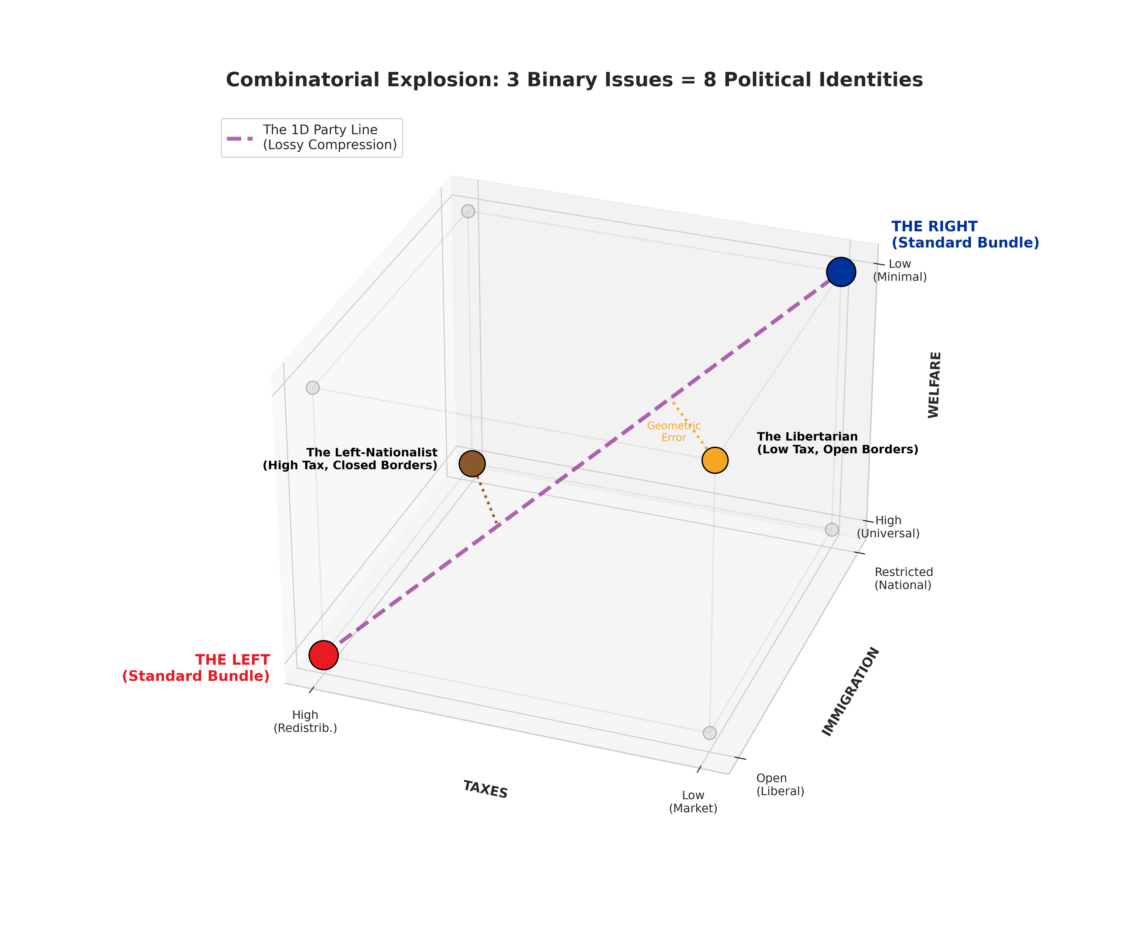
Figure 1: Three binary issues define a cube with $2^3 = 8$ corners — eight distinct political identities. A two-party system compresses this cube onto the two endpoints of a single diagonal: voters do not land somewhere along the line, they land on one of two corners. When preferences are spread across the cube this leaves 6 of the 8 positions unrepresented; voters at those orphaned corners must choose the lesser of two evils. Two caveats about the drawing. The dashed “party line” and the perpendicular “geometric error” are the continuous spatial-voting picture, drawn for legibility; the model below assigns each voter to the nearest labelled corner under Hamming distance, so the error is a jump of one edge, not a drop onto a segment. And only two of the six orphaned corners are named here — §8 is about all six.
1. Setup: Preferences as Binary Vectors
Suppose there are $n$ binary policy issues. For concreteness, take $n = 3$ — the three issues drawn in Figure 1, with the polarity fixed once and for all:
- Taxes: $1$ = low tax, $0$ = progressive wealth tax
- Welfare: $1$ = minimal welfare, $0$ = welfare expansion
- Immigration: $1$ = restricted borders, $0$ = open borders
The choice of which end is $1$ is arbitrary, but this one makes $(0,0,0)$ the coherent left position and $(1,1,1)$ the coherent right one, matching the figure.
Each voter’s preference is a binary vector $v \in \{0, 1\}^n$. With $n = 3$ issues, there are $2^n = 8$ possible preference profiles — the corners of a hypercube.
A society is a probability distribution $p$ over $\{0, 1\}^n$: the fraction of voters holding each preference profile.
Two numbers describe such a society, and the difference between them turns out to matter a great deal. The first is the support size $\lvert\operatorname{supp} p\rvert$ — how many of the $2^n$ profiles actually occur, however rare. The second is the entropy:
\[H(p) = -\sum_{v \in \{0,1\}^n} p(v) \log_2 p(v)\]Both measure “political diversity”, but not the same kind. Entropy measures how much diversity there is on average: it is small when nearly everyone agrees, even if a handful of people don’t. Support size counts the distinct positions held at all, and does not care how few people hold them. At one extreme, if everyone agrees, $p$ is concentrated on a single corner, $H(p) = 0$ and $\lvert\operatorname{supp} p\rvert = 1$. At the other, if preferences are uniform, $H(p) = n$ bits and $\lvert\operatorname{supp} p\rvert = 2^n$. In between they come apart, and §6 and §8 turn on the gap.
2. Parties as Codebooks: The Vector Quantisation View
A $k$-party system offers voters a menu of $k$ platforms $\{c_1, \ldots, c_k\} \subset \{0,1\}^n$. Each voter is assigned to the nearest party (the one matching on the most issues). This is exactly vector quantisation (VQ): we are compressing $2^n$ possible preference vectors into $k$ codewords.
The distortion of this compression is the expected Hamming distance between a voter’s true preference and their assigned party:
\[D = \sum_{v} p(v) \min_{j} d_H(v, c_j)\]where $d_H$ is the Hamming distance — the number of issues on which the voter and their party disagree.
A voter with distortion $d$ is being misrepresented on $d$ issues. This is the formal version of “the lesser of two evils.” Note that throughout, “distortion” measures distance from a voter to the nearest available platform — a representational notion — not from whichever platform ultimately wins a given election.
The choice of Hamming over Euclidean distance is not innocent. The Euclidean spatial model is the standard alternative, and how well it fits real preference data is itself contested (Thorburn et al., 2023). On binary issues Hamming is the natural metric — you either agree on an issue or you don’t, and there is no meaningful sense in which you are slightly in favour of a wealth tax.
One assumption inside it is doing a lot of work, though: Hamming charges the same for every issue. A voter with one overriding concern and two she is indifferent about is badly modelled by it. Weighted Hamming is the obvious repair, but it breaks the accounting that the rest of this post runs on — a bit is a bit, and neither entropy nor support size knows anything about salience. Decoupling distortion from the bit budget in that way is the deepest limitation of the framing here, and it is precisely the gap that intensity mechanisms such as quadratic voting exist to fill. Nothing below addresses it.
3. The Two-Party System as a 1-Bit Channel
In a two-party system ($k = 2$), the voter’s ballot carries at most 1 bit of information: Party A or Party B. (At most, not exactly — a ballot carries a full bit only if the electorate splits evenly between the two options.)
A note on vocabulary, since I will use it throughout. “Capacity” here means $\log_2$ of the number of distinct ballots a voter can cast. The ballot is a noiseless encoder with a fixed alphabet, not a noisy channel; the relevant theory is lossy source coding, not channel coding. I keep the channel metaphor because it reads well, but nothing below depends on it.
But the space of preferences has $2^n$ elements, requiring up to $n$ bits to specify. The act of voting compresses an $n$-bit preference vector into a 1-bit message — a compression that cannot be lossless unless the preferences themselves live on at most two profiles. Anything richer is being forced through too narrow a channel.
This gives us a precise criterion:
A two-party system can be lossless only when voter preferences concentrate on at most two profiles — which forces $H(p) \leq 1$ bit, but is strictly stronger.
When it works: Low-entropy electorates
Suppose 50% of voters hold preference $(0,0,0)$ (“The Left”) and 50% hold $(1,1,1)$ (“The Right”). Then:
\[H(p) = -2 \times 0.5 \log_2 0.5 = 1 \text{ bit}\]A two-party system with $c_A = (0,0,0)$ and $c_B = (1,1,1)$ achieves zero distortion — every voter is perfectly represented. The 1-bit channel suffices because the electorate only uses 1 bit of the available $n$-bit space.
This is the scenario that two-party advocates implicitly assume: that political preferences are highly correlated, clustering neatly into “Left” and “Right” bundles.
When it fails: High-entropy electorates
Now suppose voters are uniformly distributed across all 8 corners. Then $H(p) = 3$ bits and every corner is occupied, so $\log_2\lvert\operatorname{supp} p\rvert = 3$ too — the two measures coincide at this extreme. Either way the ballot’s capacity is still 1 bit. No matter how cleverly we choose $c_A$ and $c_B$, we must lose at least $3 - 1 = 2$ bits of information.
Concretely, with $c_A = (0,0,0)$ and $c_B = (1,1,1)$, consider the voter at $(1,1,0)$ — a “Libertarian” who wants low taxes and minimal welfare but open borders. There is no ballot they can cast that expresses this preference. Voting for $c_A$ actively endorses the welfare expansion they oppose; voting for $c_B$ actively endorses the closed borders they oppose. There is no third option, no way to register “I want $(1,1,0)$” — the system has no vocabulary for it. The same trap catches the voter at $(0,0,1)$, a “Left-Nationalist” who wants high taxes and strong welfare but closed borders. Each is forced not merely to accept a compromise but to cast a vote endorsing a position they reject; the information that they wanted otherwise never enters the channel.
Hamming charges 1 for this. The voter would charge more — a wrong vote cast in your name on an issue you care about is not a fraction of a grievance. Hamming is the most forgiving loss function available here; every number below is a floor, not an estimate.
The expected distortion for the uniform distribution with optimal two-party placement is:
\[D = \frac{1}{8}\sum_{v \in \{0,1\}^3} \min(d_H(v, c_A), d_H(v, c_B))\]With $c_A = (0,0,0)$ and $c_B = (1,1,1)$, the distances are:
| Voter $v$ | $d_H(v, c_A)$ | $d_H(v, c_B)$ | $\min$ |
|---|---|---|---|
| $(0,0,0)$ | 0 | 3 | 0 |
| $(0,0,1)$ | 1 | 2 | 1 |
| $(0,1,0)$ | 1 | 2 | 1 |
| $(1,0,0)$ | 1 | 2 | 1 |
| $(0,1,1)$ | 2 | 1 | 1 |
| $(1,0,1)$ | 2 | 1 | 1 |
| $(1,1,0)$ | 2 | 1 | 1 |
| $(1,1,1)$ | 3 | 0 | 0 |
On average, each voter is misrepresented on 0.75 out of 3 issues — 25% of their preferences are lost. And 6 out of 8 voter types (75%) are imperfectly represented.
One thing to be clear about before going further. Every distortion number in this post assumes the platforms are placed to minimise expected distortion — a benevolent designer running Lloyd’s algorithm on behalf of the electorate. Real parties are not benevolent designers; they are competitors trying to win. Under Downsian competition two vote-maximising parties move toward each other (Hotelling, 1929; Downs, 1957), collapsing the codebook’s spread and, in the limit, offering a 1-bit ballot that carries no policy difference at all. And in two or more dimensions no equilibrium pair of platforms generically exists (Plott, 1967; McKelvey, 1976), so “optimal two-party placement” is not a prediction about any actual political system. Real distortion is worse than the numbers here — another sense in which this analysis is a lower bound.
4. The General Rate–Distortion Tradeoff
More generally, a $k$-party system provides $R = \log_2 k$ bits of representation. The relationship between rate and distortion is governed by rate–distortion theory.
For a uniform source over $\{0,1\}^n$ with Hamming distortion, the rate–distortion function is:
\[R(D) = n\left(1 - H_b\!\left(\frac{D}{n}\right)\right)\]where $H_b(x) = -x\log_2 x - (1-x)\log_2(1-x)$ is the binary entropy function. (The argument is $x$, not $p$; $p$ is already spoken for as the electorate distribution from §1.) Read forwards, the theorem says you need at least $R(D)$ bits — at least $2^{R(D)}$ parties — to achieve distortion $D$. Read backwards, it says what distortion a given number of parties permits.
It is worth doing both and comparing:
| Parties ($k$) | Bits ($R$) | Exact optimum, $n=3$ | $D$ permitted by $R(D)$ |
|---|---|---|---|
| 2 | 1 | 0.75 | 0.522 |
| 4 | 2 | 0.5 | 0.185 |
| 8 | 3 | 0 | 0 |
The third column is the exact optimum over all codebooks of size $k$ at $n = 3$, found by brute force. The fourth is what asymptotic rate–distortion theory says is achievable at that rate. The gap is large, and it is not slack in the analysis: closing it would require coding many voters jointly into a single codeword, which no ballot can do, since every voter must independently select from the same fixed menu. Rate–distortion theory gives a valid lower bound on the distortion of a $k$-party system, but a badly loose one at $n = 3$. The theory that actually applies here is one-shot vector quantisation, not Shannon’s asymptotic result. To reach zero distortion with $n$ binary issues you need $k = 2^n$ parties — one for every corner of the hypercube.
5. The Curse of Dimensionality
The table above reveals the fundamental problem: the number of parties required for lossless representation grows exponentially in the number of issues.
For $n = 3$, we need 8 parties — manageable. But for $n = 10$ issues, we need $2^{10} = 1{,}024$ parties. For $n = 30$:
\[2^{30} \approx 1 \text{ billion parties}\]This is the curse of dimensionality applied to governance. No ballot can present a billion options. The cognitive and institutional costs make this impossible — not, note, because $2^n$ options is impossible (a ballot with $n$ checkboxes offers exactly that many) but because $2^n$ mutually exclusive menu items is. §6 turns on that distinction.
This creates a dilemma:
- Few parties ($k = 2$): Low cognitive cost, but high distortion — voters are systematically misrepresented.
- Many parties ($k \to 2^n$): Low distortion, but impossible cognitive and institutional overhead.
We cannot “party” our way out of this problem.
A parliamentary system is a partial exception worth naming, and living under MMP I should name it. What a coalition government outputs is not one of $k$ platforms but a negotiated programme, and the set of feasible coalition programmes is combinatorially larger than the set of parties — so the effective codebook is bigger than $\log_2 k$ suggests. But the enlargement is not voter-controlled. Bargaining raises the system’s representational capacity while lowering each voter’s control over which codeword they end up getting, and the ballot they actually cast still carries $\log_2 k$ bits. That is a real distinction, and one this framework can express: capacity and control are separate things, and coalitions trade one for the other.
6. Matching Structure: The Right Factorisation
How hard the curse bites depends on how much of the cube the electorate actually occupies. If voter preferences are highly correlated, most of the $2^n$ corners are empty and a small number of parties suffices. The curse bites when the occupied corners are spread out — when knowing a voter’s position on taxes tells you little about where they sit on immigration, so that most of the cube is populated. Statistical independence across issues is the cleanest way to get there, but it is not required: what matters is how many distinct profiles occur, and a population can fill the cube without any of its issues being independent.
In the extreme “impartial culture” model (uniform distribution) all $2^n$ corners are occupied and the full exponential cost is unavoidable. Real electorates lie somewhere between these extremes, but any substantial spread across the cube pushes the required number of parties above what is practical.
Critically, the causal direction matters. If voters’ preferences appear correlated because the party system only offers correlated bundles, then the observed low entropy is an artifact of the compression, not a property of the underlying preferences. The system may be manufacturing the conformity it relies on.
Real electorates do have structure, though: knowing a voter’s position on healthcare predicts their position on taxes; knowing their position on immigration tells you something about drug policy. Preferences cluster. This reframes the question. The right thing to ask is not “bundle or unbundle?” but what factorisation of the ballot matches the conditional-independence structure of voter preferences? Two parties is the extreme of forcing everything onto a single axis. Issue-by-issue is the extreme of treating every dimension as independent.
Before making that concrete, two quantities have to be kept apart, because conflating them is where most reform arguments go wrong. If you want every voter represented exactly, the ballot needs $\log_2\lvert\operatorname{supp} p\rvert$ bits — the log of the number of distinct preference profiles that actually occur, however rare each one is. If you only want average fidelity, $H(p)$ is the right budget, and Shannon’s source coding theorem says you can approach it. But the gap between the two is not a rounding error: it is exactly the tail. Take an electorate that puts 99% of its mass on $(0,0,0)$ and scatters the remaining 1% over the other seven corners. Its entropy is 0.109 bits — a two-party ballot has nine times the capacity it seems to need — and yet that ballot still misrepresents one voter in a hundred, and it takes all eight platforms to represent everyone. A ballot designed to $H(p)$ is a ballot that has decided in advance which minorities to drop. So:
To represent every voter exactly, the ballot’s capacity must be at least $\log_2\lvert\operatorname{supp} p\rvert$ — and its factorisation should match the conditional-independence structure of $p$.
§3 already gave the two extremes. When the electorate sits on two corners, two parties are exactly right, and issue-by-issue voting extracts three bits to carry one — the other two are pure overhead. When the electorate is spread uniformly over all eight, two parties discard a quarter of every voter’s preferences, four parties still discard a sixth, and only a ballot with all $2^n$ options reaches zero. Both are special cases of one principle, and the interesting case is the one in between.
It is worth being honest about how cheap the second of those claims is. Under the definition in §2, distortion is distance to your nearest available platform, so a ballot that lets you name any vector achieves zero distortion for any $p$ whatsoever. That is a fact about the definition, not a discovery about direct democracy. What §2’s distortion measures is how much of a preference a ballot can carry — expressiveness — not how well the resulting government governs. §8 comes back to that distinction.
6.1 The clustered electorate: factor along the clusters
Consider 6 issues that split into two thematic clusters:
- Economic axis: {wealth tax, welfare expansion, public healthcare}
- Social axis: {drug liberalisation, immigration, surveillance}
Within each cluster, issues are tightly correlated. Across clusters they are independent — your economic leanings tell us nothing about your social ones.
Concretely, say each cluster is split 50/50 between its all-Yes corner and its all-No corner, with the two clusters drawn independently. The electorate has 4 equally-sized types:
| Type | Economic | Social |
|---|---|---|
| Progressive-libertarian | $(1,1,1)$ | $(1,1,1)$ |
| Progressive-authoritarian | $(1,1,1)$ | $(0,0,0)$ |
| Conservative-libertarian | $(0,0,0)$ | $(1,1,1)$ |
| Conservative-authoritarian | $(0,0,0)$ | $(0,0,0)$ |
Four equally likely types, so $H(p) = \log_2\lvert\operatorname{supp} p\rvert = 2$ bits — the two criteria agree here, as they always do when the occupied profiles are equally weighted.
| Mechanism | Bits/voter | Distortion (out of 6) |
|---|---|---|
| 2 parties (single axis) | 1 | 1.5 |
| 4 parties (one per type) | 2 | 0 |
| 6 issue-by-issue votes | 6 | 0 |
| 2 cluster bundles | 2 | 0 |
Two parties fail because forcing 4 types onto one axis collapses the orthogonal dimension. Issue-by-issue succeeds but extracts 4 bits more than the source contains. The clean answer is to ask each voter for two bits — a single Y/N for the economic package and a single Y/N for the social package — yielding zero distortion at exactly the two bits the electorate contains.
6.2 The principle
The right ballot mirrors the conditional-independence graph of voter preferences. Bundle issues that travel together; separate clusters that don’t. The voter transmits one bit per cluster — not one bit per electorate, and not one bit per issue.
Survey data on real political opinion typically finds two to four dominant axes of variation, not 1 (the two-party assumption) and not 30 (the impartial-culture assumption). That is suggestive rather than decisive, and it is worth saying why: the number of principal components is not a count of bits, and it is certainly not a bound on support size. An electorate can load almost all of its variance on two components and still occupy every corner of the cube. What the survey evidence does suggest is that the coupling structure is coarse — a few blocks of issues that move together — which is the input the factorisation argument needs. It does not by itself license a small menu.
Liquid Democracy falls out as a plausible refinement. If voters can delegate per-cluster, they import a more informed codebook for dimensions they don’t follow while voting directly on those they do. The total representation is a composite across clusters, rather than a single lossy codeword that bundles everything. Note, though, that this argument leaves the pure-preference frame the rest of the post lives in: delegation helps only if there are facts about a policy domain that a delegate knows better, not merely preferences. Nobody knows your preferences better than you do. That is a different — and contestable — model of what voting is for.
Two further caveats, both of which I think are more serious than they look.
First, factoring the ballot to match $p$ requires knowing $p$’s conditional-independence structure, and the ballot is the only instrument we have for measuring it. Worse, the endogeneity point above says the instrument distorts what it measures: a two-party ballot returns two-party-shaped data. The recommendation and the diagnosis are entangled. This is not fatal, but it is the hard part, and it is the problem I take up in a later post, which estimates the dependency graph from Polis-style agree/disagree votes and reads the ballot off the estimate. That treatment is sharper than this one: it separates separability-distortion (from deciding coupled issues in separate questions) from menu-distortion (from offering fewer combinations than voters want), and shows that the cost of a faithful ballot is exponential only in the dependency graph’s treewidth, not in the size of its coupled blocks.
Second, I have assumed throughout that voters report their preferences honestly. Gibbard–Satterthwaite guarantees that no non-trivial deterministic voting rule is strategyproof, and a per-cluster ballot with a known aggregation rule is manipulable like any other — reporting a profile is less manipulable than choosing among outcomes, but it is not immune. Expressiveness and strategyproofness are different problems, and this post is only about the first.
7. The Limits of Unbundling: The Paradox of Multiple Elections
The mistake at both extremes is the same: imposing a structure that doesn’t match the electorate. Two-party democracy assumes one axis; pure direct democracy assumes none. Both are wrong in the same way, in opposite directions — and the second failure has a name.
There is an assumption hiding inside the case for unbundling in §6: that a voter’s satisfaction is the sum of per-issue agreements. This is the separability assumption, and it is what makes Hamming distortion the right loss function.
Real preferences are often non-separable. A natural example:
I support expanding welfare for families, jobseekers, and the disabled. Unless a UBI is on the table — in which case I support the UBI and reject the targeted increases.
The preference between “expand targeted welfare” and “leave it alone” is conditional on whether UBI passes. Voting on each issue independently can produce UBI and the targeted increases — a package nobody actually wanted. This is the case Lacy & Niou (2000) make against issue-by-issue referendums, and remains the canonical treatment of non-separable preferences in that setting.
The textbook version is the paradox of multiple elections (Brams, Kilgour & Zwicker, 1998), also called the compound-majority or multiple-election paradox. Three blocs vote on three issues:
| Bloc | Share | Bundle |
|---|---|---|
| A | 40% | $(Y, Y, N)$ |
| B | 30% | $(Y, N, Y)$ |
| C | 30% | $(N, Y, Y)$ |
Issue-by-issue majorities give Y (70%), Y (70%), Y (60%) — outcome $(Y, Y, Y)$, a bundle no voter actually preferred. Each voter sits at Hamming distance 1, which looks fine under separable loss but is catastrophic if voters care about coherent packages over per-issue marginals.
This is not Ostrogorski’s paradox, though the two are routinely confused. Ostrogorski’s is about parties: a party preferred by a majority of voters — each backing whichever party agrees with them on more issues — nonetheless loses on a majority of the issues, or the reverse. There are no parties in the example above. Daudt & Rae (1976) is the standard reference for that case.
Does the §6 framework rescue us? Partly. Non-separability and statistical dependence are related but not the same thing: the first is a property of an individual’s preference ordering, the second a property of the population’s distribution over top choices. Non-separable preferences usually induce dependence — a voter who wants exactly one of UBI and targeted welfare never lands on the $(1,1)$ corner — so the §6.2 diagnostic will often catch it. But it can be fooled. An electorate in which every voter is non-separable can still show perfectly independent marginals, provided different voters are non-separable in different directions: mix four types, each excluding a different corner of $\{0,1\}^2$, and the population’s top choices are uniform over all four. Correlation between ballots is evidence of coupling; the absence of correlation is not proof of its absence.
The deeper problem is that the diagnostic is a correlation test on observed ballots, and non-separability lives in counterfactual structure — what I would want if the other measure passed — that observed ballots do not contain. You cannot recover a CP-net from marginal correlations. Detecting non-separability properly means eliciting conditional preferences, which is a strictly harder measurement problem than anything else in this post.
So the honest version is weaker than I would like: the right factorisation usually keeps coupled issues bundled, and the paradox usually does not arise. “Usually” is doing real work in that sentence.
None of this is new, and §6.2’s principle is a rediscovery rather than an invention. Representing conditional preference structure as a graph is the central idea of the CP-net literature (Boutilier et al., 2004), and the cost of deciding coupled issues by sequential per-issue votes is exactly the subject of Lang & Xia (2009) and Ahn & Oliveros (2012). Worth saying, since it costs nothing and the field got there first.
8. The Right to Be Heard
So far we’ve framed compression loss as average distortion — how much voters’ preferences fail to match the system’s output. But averages hide a sharper question: whose preferences are lost?
Lossy compression doesn’t lose information uniformly. It loses the information furthest from the codebook. In a two-party system with platforms on the principal axis, the silenced voters are exactly those at the off-diagonal corners of the cube: libertarians (low tax, low welfare, open immigration), left-nationalists (high tax, strong welfare, closed borders), eco-socialists, religious progressives — voters whose combination of concerns doesn’t lie on the dominant ideological axis. These are not random voters. They are systematically the people whose particular bundle crosses the lines the dominant axis was drawn to separate.
This is the structural source of misrepresentation — not disenfranchisement in the strict sense, since nobody is denied a vote; what they are denied is a vote that says what they mean. When a voter says “no party represents me,” they are usually right. Their preference profile sits in a region of the cube that no codeword covers, and by construction the system cannot recover it. The feeling is not paranoia — it is the predictable consequence of routing an $n$-bit signal through a 1-bit ballot.
The model also says something about who this happens to, but something narrower and sharper than “minorities lose.” Distortion-minimising codebooks chase mass: any off-axis cluster large enough to be worth a platform will eventually get one, whether by design or by electoral competition. What the geometry guarantees is that the persistently misrepresented are the numerically small, off-axis clusters — small enough that no competitor gains by moving toward them, and cross-cutting enough that neither existing platform covers them. Whether those clusters coincide with demographic minorities is an empirical question, not a theorem; plenty of majority-group voters sit off the axis too. But there is a reason to expect the overlap is common: a group whose distinctive policy concerns cut across the dominant cleavage is by construction off-axis, and being small is part of why the cleavage got drawn somewhere else in the first place.
This reframes the central question. Instead of “is the system efficient?” we should ask: does every voter have the right to transmit their preferences without distortion? A democracy that meets that standard must offer a ballot with capacity at least $\log_2\lvert\operatorname{supp} p\rvert$ — enough distinct options to cover every preference profile anyone actually holds, however few hold it. Matching $H(p)$ is not enough. Entropy is the budget for average fidelity, and the voters it spends first are precisely the ones in the tail: the right-to-be-heard standard is the support criterion, not the entropy criterion. Anything less is a system that, by design, silences someone — and has chosen in advance who.
One caveat worth stating plainly. The right argued for here is informational — the right to be heard. It is distinct from the right to be obeyed. Even under perfect issue-by-issue voting the minority loses on each issue; their preferences are recorded but not enacted. The information-theoretic argument tells you what it takes to register every voter’s preferences faithfully. Whether the system then aggregates them fairly — proportionally, via Condorcet, via supermajority on sensitive issues — is a separate question. But registering is the prerequisite. A democracy that cannot even hear its minorities cannot meaningfully claim to weigh them.
Summary
| Electorate | Profiles actually held | Optimal ballot | Bits/voter |
|---|---|---|---|
| Aligned (one axis) | $2$ | 2 parties | 1 |
| Clustered ($c$ binary axes) | $2^c$ | $c$ cluster-bundles (or $2^c$ parties) | $c$ |
| Independent (every corner occupied) | $2^n$ | Issue-by-issue | $n$ |
| Arbitrary $p$ | $\lvert\operatorname{supp} p\rvert$ | Match the factorisation | $\log_2\lvert\operatorname{supp} p\rvert$ |
The mathematics is simple. Preferences over $n$ binary issues live in an $n$-dimensional space, but the effective dimensionality is $\log_2\lvert\operatorname{supp} p\rvert$ — the log of how many profiles the electorate actually holds. A ballot with less capacity than that cannot represent everyone; more than that wastes voter effort. ($H(p)$ is the corresponding figure if you only care about the average voter. It is always smaller, and the difference is exactly the tail.) Two parties is right when the electorate is one-dimensional. Pure issue-by-issue is right when issues are independent. Neither is universally right — and the universal answer is to factor the ballot to match the conditional-independence structure of preferences, bundling within clusters and separating across them.
The deeper point is not efficiency but whose voice the channel can carry. Every voter whose preferences lie off the codebook’s principal axes is, by construction, silenced — and these are not random voters, but the predictable ones: the small, cross-cutting clusters whose particular bundle of concerns the dominant axis was drawn to ignore. A democracy that takes representation seriously owes its citizens a ballot wide enough to hear them. We don’t need to choose between bundling and unbundling. We need a mechanism that can do either, dimension by dimension — and that owes a hearing to everyone, not just the median voter.
References
- Thorburn et al. (2023). Error in the Euclidean Preference Model. arxiv.org/abs/2208.08160
- Brams, S., Kilgour, D. M. & Zwicker, W. (1998). The paradox of multiple elections. Social Choice and Welfare 15(2):211–236.
- Lacy, D. & Niou, E. (2000). A problem with referendums. Journal of Theoretical Politics.
- Daudt, H. & Rae, D. (1976). The Ostrogorski paradox: a peculiarity of compound majority decision. European Journal of Political Research.
- List, C. & Pettit, P. (2002). Aggregating sets of judgments: an impossibility result. Economics and Philosophy.
- Boutilier, C., Brafman, R., Domshlak, C., Hoos, H. & Poole, D. (2004). CP-nets: a tool for representing and reasoning with conditional ceteris paribus preference statements. Journal of Artificial Intelligence Research.
- Lang, J. & Xia, L. (2009). Sequential composition of voting rules in multi-issue domains. Mathematical Social Sciences.
- Ahn, D. S. & Oliveros, S. (2012). Combinatorial voting. Econometrica.
- Hotelling, H. (1929). Stability in competition. The Economic Journal.
- Downs, A. (1957). An Economic Theory of Democracy. Harper & Row.
- Plott, C. (1967). A notion of equilibrium and its possibility under majority rule. American Economic Review.
- McKelvey, R. (1976). Intransitivities in multidimensional voting models and some implications for agenda control. Journal of Economic Theory.
- Cover, T. & Thomas, J. (2006). Elements of Information Theory, 2nd ed. (Chapter 10, Rate–Distortion Theory.)
Comments