Typicality
In high dimensions, typical is unintuitive
August 10, 2024
What is likely is not (necessarily) typical.
Let’s start with a motivating example: We have a biased coin $p(\text{Heads}) = 0.8$ which we flip $n=100$ times. The most likely outcome is 100 heads, with probability $0.8^{100}=2.037036 \times 10^{-10}$, a small number. So the vast majority of the time, we will observe something else. Most of these other outcomes will be in the range of 70-90 heads. We call these outcomes ‘typical’.
Using the Binomial distribution, we can calculate and plot the probability of getting k heads as;
\[p(k) = \left( 100 \; \text{choose} \; k \right)0.8^k0.2^{100-k}\]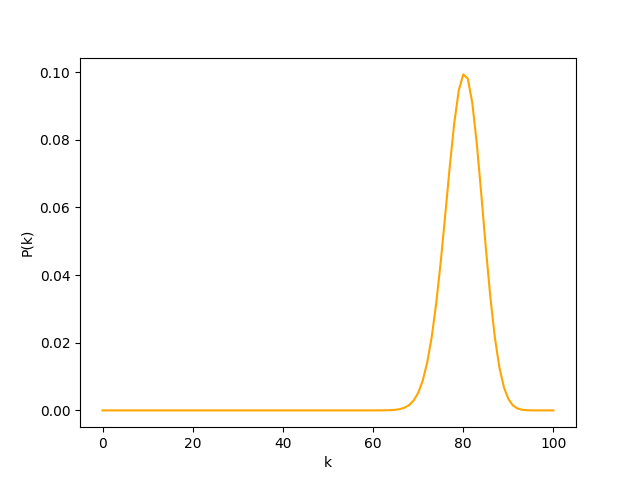
The potentially counter intuitive part being that each individual outcome (with ~70-90 heads) is less likely than 100 heads, yet, they are the ones we observe.
The explanation is that there is only 1 way to get 100 heads, but MANY ways to get (say) 80 heads ($100 \; \text{choose} \; 80 = 5.3598337 \times 10^{20}$).
Definition (for discrete random variables)
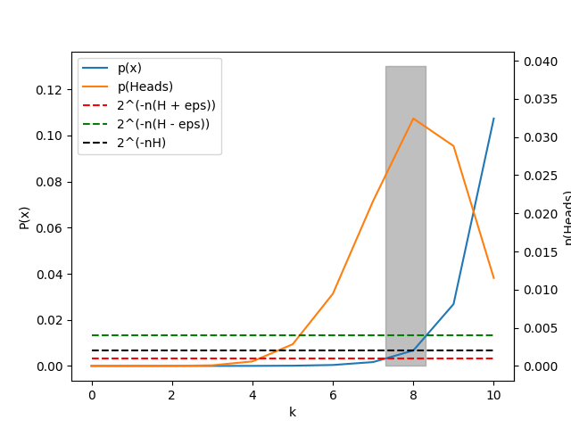
The typical set $\mathcal T (p(x))_{\epsilon}$ is the set of sequences $(x_1,x_2,…,x_n) \in X_n$ with the property
\[2^{−n(H (X)+\epsilon)} \le p(x_1,x_2,...,x_n) \le 2^{−n(H (X)-\epsilon)} \\\]From (Cover & Thomas, 2006) page 59.
So for our coin flipping example, let’s pick $\epsilon = 0.1$ and calculate the typical set. (We drop to $n=10$ flips here, purely so the individual outcomes are still visible on a plot.)
A more practical example; a survey.
We have a survey with 100 binary questions.
- Do you consider yourself to be a morning or night person?
- Do you prefer cats or dogs?
- Do you prefer tea or coffee?
- Do you prefer to read or watch TV?
- Do you vote left or right?
- … etc
We can collect the data, and we may see that;
- 60% of people consider themselves to be morning people
- 70% of people prefer dogs
- 80% of people prefer coffee
- 60% of people prefer to read
- 30% of people vote left
- etc…
From this data we can construct an archetype of a person who took the survey. This person would be a morning person, prefer dogs, prefer coffee, prefer to read, and vote right. This person is the most likely person to have taken the survey. But they are unlikely to exist! And may not be a good representation of the people who took the survey.
If we rearrange the definition of discrete typical sets, we can find a close connection to the definition of entropy.
\[\begin{align*} 2^{−n(H (X)+\epsilon)} &\le p(x_1,x_2,...,x_n) \le 2^{−n(H (X)-\epsilon)} \tag{typical set} \\ H (X)-\epsilon &\le -\frac{1}{n} \log p(x_1,x_2,...,x_n) \le H (X)+\epsilon \tag{log both sides} \\ -\frac{1}{n} \log \prod_{i=1}^n p(x_i) &= -\frac{1}{n} \log p(x_1,x_2,...,x_n) \tag{independence} \\ &= -\frac{1}{n} \sum_{i=1}^n \log p(x_i) \\ H(X) &= \lim_{n \to \infty} -\frac{1}{n} \sum_{i=1}^n \log p(x_i) \tag{AEP} \\ &= - \sum_{x \in X} p(x) \log p(x) \tag{entropy} \end{align*}\]Assuming each $x_i$ in the sequence is independent and identically distributed (i.i.d) from $p(x)$.
AEP is the asymptotic equipartition property, which states that for sequences of i.i.d random variables, the mean log probability converges to the entropy of the distribution (Cover & Thomas, 2006) page 58.
Definition (for continuous random variables)
The typical set $\mathcal T (p(x))_{\epsilon}$ is the set of sequences $(x_1,x_2,…,x_n) \in X_n$ with the property
\[\mid - \frac{1}{N} \log p(x) - h(X) \mid \le \epsilon\]Where $h(x)$ is the differential entropy of $p(x)$. (Cover & Thomas, 2006) page 245.
Let’s work through a continuous example. A d-dimensional isotropic Gaussian distribution.
First, we can reframe a d-dimensional Gaussian as sequence of $d$ i.i.d 1D Gaussians. For example, if $d=3$ then we can sample 3 times from a 1D Gaussian to get a sample from a 3D Gaussian.
\[\begin{align*} p(x) &= \prod_{i=1}^d \mathcal N(x_i; 0, \sigma^2) \\ \mathcal N(x; 0, \sigma^2 I) &= \frac{1}{(2\pi \sigma^2)^{1/2}} \exp \left( -\frac{1}{2\sigma^2} x^2 \right) \\ \end{align*}\]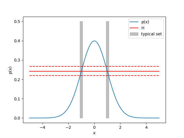
This doesn’t seem to make much sense in 1 dimension. But in higher dimensions, it’s easier to imagine. If I sample $d$ times from a Gaussian, what’s the chance I get all zeros? Very small. Instead, I’m likely to sample some small numbers, and a few larger numbers. Each coordinate contributes about $\sigma^2$ to the squared norm, so the sample lands near the sphere of radius $\sqrt d \sigma$. Thus the typical set is a thin shell around that sphere — not around the origin, and (note) not around the unit sphere either; the radius grows with dimension. This is also known as the Gaussian Annulus Theorem.
For a d-dimensional spherical Gaussian with unit variance in each direction, for any $\beta \le \sqrt{d}$, all but at most $3e^{−c\beta^2}$ of the probability mass lies within the annulus $\sqrt{d} - \beta \le |x| \le \sqrt{d} + \beta$, where c is a fixed positive constant.
So high dimensional Gaussian distributions can be imagined as hollow spheres, rather than the bell shaped curves we are used to in 1D.
Much like our discrete example (but replace probability mass with probability density and binomial counts with volume), the most likely outcome has small probability density. And as we move outward, the volume increases exponentially. Thus even though the probability density is small, the volume is large, and we are likely to observe points in this region.
Two things ‘typical’ can mean
Worth pulling apart, because most treatments skip it and it matters more than it looks.
Look again at the definition. It says the typical set is where $-\frac1n \log p$ sits close to $h$. That is a statement about the density: every member of the set is roughly as probable as every other. Call that the level set property, or equipartition — it is the EP in AEP.
But the reason we care about the typical set is usually different. We care because it is where the samples are: it captures nearly all the probability mass, in nearly the smallest volume that could. Call that the high-probability set property.
For sequences of i.i.d. draws these are two descriptions of the same object, which is why the distinction rarely comes up. They are not the same thing in general. Cover and Thomas devote a section to it (Cover & Thomas, 2006) (§3.3): the typical set and the genuinely smallest high-probability set have the same size to first order in the exponent, but they are different sets.
Where this bites: push a distribution through a diffeomorphism — a neural flow, say — and the change of variables preserves one of these properties exactly and wrecks the other.
- High-probability: preserved exactly by any diffeomorphism, because mass is conserved under a bijection. If a set holds 95% of the source’s mass, its image holds 95% of the target’s, with no conditions at all.
- Level set: not preserved, because the density gets rescaled by the Jacobian determinant, which varies from point to point. Two points sitting on the same level set in the source come out with different densities in the target.
They coincide only when $\lvert \det J \rvert$ is constant. So if you find yourself saying “the typical set” about a distribution defined by a flow, it is worth knowing which of the two you meant.
A caveat about sequences
I have been sloppy above, in a way worth being explicit about.
The classical typical set is defined over a sequence of $n$ i.i.d. draws from $p$. The AEP is what makes it non-empty and well-behaved, and the AEP needs that i.i.d. assumption. But people routinely talk about the typical set of, say, a distribution over images — where $x$ is a single image and the pixels are emphatically not i.i.d. There is no sequence and there is no $n \to \infty$.
The Gaussian example above hides this, because for an isotropic Gaussian the two readings coincide: a $d$-dimensional isotropic Gaussian genuinely is a sequence of $d$ i.i.d. 1-D Gaussians, which is why I could reframe it that way. That trick works for exactly this one case and breaks for every interesting distribution.
So what is actually being assumed in the image case? Not the AEP. Something weaker:
$-\frac{1}{d}\log p(X)$ concentrates around $\frac{1}{d}h(X)$.
That is, if you draw real data and compute its per-dimension log density, you get a narrow distribution. This is what makes “typical” a meaningful category. It is implied by the AEP in the i.i.d. case, but it can hold for all sorts of dependent structure, and it can also fail.
The useful thing about stating it this way is that it is an empirical claim about your data and your density model, and you can just go and check it. Train a flow, compute $-\frac1d \log p(x)$ on held-out data, plot the histogram:
- If it’s tight, typicality is a meaningful category for that data, and you should set $\epsilon$ from the observed spread — say the 5th to 95th percentile band — rather than picking a number.
- If it’s broad, the typical set is nearly everything, and any method built on it isn’t doing much work.
This is the same measurement used to test whether an input is out-of-distribution (Nalisnick et al., 2019), where it was found that raw likelihood is a poor OOD signal but the typicality statistic is a much better one (Nalisnick et al., 2019).
Where this went
I spent a while trying to use typicality as a constraint for solving inverse problems — the idea being that if MAP returns the mode, and the mode is atypical, then perhaps we should ask for the most likely solution that is also typical. That work outgrew a blog post and now lives at github.com/act65/pits. It is unfinished, and the “two things typical can mean” section above turned out to be the crux of it.
These ideas were developed while studying at VUW with Bastiaan Kleijn and Marcus Frean. I was funded by GN.
Bibliography
- Cover, T. M., & Thomas, J. A. (2006). Elements of Information Theory (2nd ed.). Wiley-Interscience. https://www.wiley.com/en-us/Elements+of+Information+Theory%2C+2nd+Edition-p-9780471241959
- Nalisnick, E., Matsukawa, A., Teh, Y. W., & Lakshminarayanan, B. (2019). Detecting Out-of-Distribution Inputs to Deep Generative Models Using Typicality. https://arxiv.org/abs/1906.02994
- Nalisnick, E., Matsukawa, A., Teh, Y. W., Gorur, D., & Lakshminarayanan, B. (2019). Do Deep Generative Models Know What They Don’t Know? International Conference on Learning Representations (ICLR). https://arxiv.org/abs/1810.09136
Comments