A Tutorial on Itô's Lemma
July 22, 2025
In the world of deterministic calculus, the chain rule is a cornerstone for differentiating composite functions. However, when we step into the realm of stochastic processes, particularly those involving Brownian motion (or Wiener processes), the familiar rules of calculus need a significant adjustment. This tutorial will guide you through why the standard chain rule isn’t sufficient for Stochastic Differential Equations (SDEs) and introduce Itô’s Lemma, the stochastic counterpart, along with derivations of common differentiation rules.1
1. Why Does the Standard Chain Rule Fail for SDEs?
The heart of the issue lies in the peculiar nature of Brownian motion, denoted $ \beta(t) $ (or $ W(t) $). Unlike the smooth, predictable paths of deterministic functions, Brownian motion exhibits unique properties:
- Continuous but Nowhere Differentiable: A path of Brownian motion is continuous everywhere, but it’s so “wiggly” or “jagged” that it’s impossible to define a unique tangent (derivative) at any point in the standard calculus sense. Its “derivative,” often called white noise, is not a regular function.
- Non-Negligible Quadratic Variation: This is the critical difference. In ordinary calculus, when we consider a small change $ \Delta t $, the square of that change, $ (\Delta t)^2 $, becomes negligible much faster than $ \Delta t $ itself as $ \Delta t \to 0 $. For Brownian motion, the square of a small increment $ \Delta\beta_t = \beta(t + \Delta t) - \beta(t) $ behaves differently.
Let’s look at the “Itô multiplication rules” for infinitesimals $ dt $ (a small change in time) and $ d\beta_t $ (a small increment of a standard Wiener process, where $ E[d\beta_t] = 0 $ and $ E[(d\beta_t)^2] = dt $):
- $ (dt)^2 \to 0 $
- As in ordinary calculus, the square of an infinitesimal time step is of a higher, negligible order.
- $ dt \cdot d\beta_t \to 0 $
- The product of a deterministic infinitesimal and a stochastic one is also of a higher, negligible order. More formally, $ E[dt \cdot d\beta_t] = dt \cdot E[d\beta_t] = 0 $, and $ Var(dt \cdot d\beta_t) = (dt)^2 Var(d\beta_t) = (dt)^2 dt = (dt)^3 $. The typical magnitude $ (dt)^{3/2} $ vanishes faster than $ dt $.
- $ (d\beta_t)^2 \to dt $
- This is the game-changer! The square of an infinitesimal increment of Brownian motion is not zero in the limit. Instead, it is equivalent to an infinitesimal increment of time $ dt $. This comes from $ E[(d\beta_t)^2] = Var(d\beta_t) + (E[d\beta_t])^2 = dt + 0^2 = dt $.
The Implication for Taylor Expansions: The standard chain rule is derived from a first-order Taylor expansion: \(df \approx \frac{\partial f}{\partial t}dt + \frac{\partial f}{\partial x}dx\) This expansion ignores second-order terms like $ (1/2)\frac{\partial^2 f}{\partial x^2}(dx)^2 $ because, in ordinary calculus, $ (dx)^2 $ (where $ dx $ is a change in a deterministic variable) is of a higher order (e.g., $ (dt)^2 $) and vanishes faster.
However, if $ x $ is an Itô process, say $ dX_t = a dt + b d\beta_t $, then: \((dX_t)^2 = (a dt + b d\beta_t)^2 = a^2(dt)^2 + 2ab dt d\beta_t + b^2(d\beta_t)^2\) Using the Itô multiplication rules, this simplifies to: \((dX_t)^2 = a^2(0) + 2ab(0) + b^2(dt) = b^2 dt\)
Since $ (dX_t)^2 $ is of order $ dt $, the term $ (1/2)\frac{\partial^2 f}{\partial X^2}(dX_t)^2 = (1/2)\frac{\partial^2 f}{\partial X^2}b^2 dt $ is also of order $ dt $. It’s of the same order of magnitude as the first-derivative terms and therefore cannot be ignored.
This non-negligible contribution from the squared stochastic increment means the ordinary chain rule, which omits these second-order effects, will give incorrect results for functions of Itô processes.
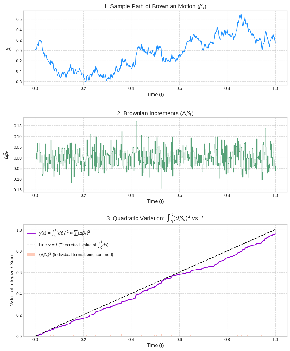
Figure 1: A SDE simulated with n=500. The $ \sum \Delta $s converges to linear with increasing n.
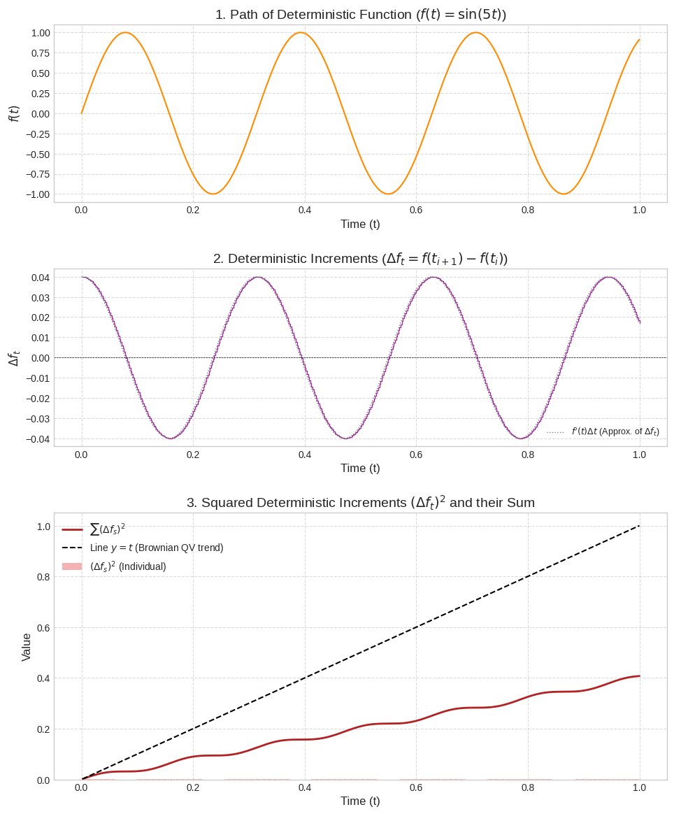
Figure 2: An ODE simulated with n=500. The $ \sum \Delta $s converges to zero with increasing n.
2. Introducing Itô’s Lemma: The Stochastic Chain Rule
Itô’s Lemma provides the correct way to differentiate a function $ f(t, X_t) $ where $ X_t $ is an Itô process defined by the SDE:2 \(dX_t = a(t, X_t) dt + b(t, X_t) d\beta_t\)
Itô’s Lemma states: The differential $ df(t, X_t) $ is given by: \(df = \left[ \frac{\partial f}{\partial t} + a(t, X_t)\frac{\partial f}{\partial X} + \frac{1}{2}b(t, X_t)^2\frac{\partial^2 f}{\partial X^2} \right] dt + b(t, X_t)\frac{\partial f}{\partial X} d\beta_t\)
Notice the extra term: $ \frac{1}{2}b(t, X_t)^2\frac{\partial^2 f}{\partial X^2} dt $. This is the “Itô correction term” and it arises directly from the $ (d\beta_t)^2 \to dt $ rule. It accounts for the non-negligible quadratic variation of the stochastic process $ X_t $.
If the function $ f $ depends on time and two Itô processes, $ X_t $ and $ Y_t $, where: $ dX_t = a_X dt + b_X d\beta_t $ $ dY_t = a_Y dt + b_Y dW_t $ and $ d\beta_t dW_t = \rho dt $ (where $ \rho $ is the correlation between the Wiener increments), then Itô’s Lemma for $ f(t, X_t, Y_t) $ is: \(df = \frac{\partial f}{\partial t}dt + \frac{\partial f}{\partial X}dX_t + \frac{\partial f}{\partial Y}dY_t + \frac{1}{2}\frac{\partial^2 f}{\partial X^2}b_X^2 dt + \frac{1}{2}\frac{\partial^2 f}{\partial Y^2}b_Y^2 dt + \frac{\partial^2 f}{\partial X \partial Y}b_X b_Y \rho dt\)
3. Deriving Differentiation Rules
Let $ X_t $ and $ Y_t $ be Itô processes: $ dX_t = a_X dt + b_X d\beta_t $ $ dY_t = a_Y dt + b_Y dW_t $ Assume for simplicity in the product and quotient rules that $ d\beta_t $ and $ dW_t $ are increments of the same standard Wiener process, so $ d\beta_t dW_t = (d\beta_t)^2 = dt $. Thus, the quadratic covariation term $ dX_t dY_t = b_X b_Y dt $.
3.1 The Sum Rule
Ordinary Calculus: $ d(X + Y) = dX + dY $
Stochastic Calculus (using Itô’s Lemma): Let $ f(X_t, Y_t) = X_t + Y_t $.
- $ \frac{\partial f}{\partial X} = 1 $, $ \frac{\partial f}{\partial Y} = 1 $
- All second derivatives are 0. Applying Itô’s Lemma (for a function of two processes, with $ \frac{\partial f}{\partial t}=0 $): \(d(X_t + Y_t) = (1)dX_t + (1)dY_t + \frac{1}{2}(0)(dX_t)^2 + \frac{1}{2}(0)(dY_t)^2 + (0)dX_t dY_t\) $ d(X_t + Y_t) = dX_t + dY_t $
Result: The sum rule is the same in both ordinary and Itô calculus. This is because the sum function is linear, and the Itô correction terms involve second derivatives, which are zero for linear functions.
3.2 The Product Rule
Ordinary Calculus: $ d(XY) = Y dX + X dY $
Stochastic Calculus (Itô Product Rule): Let $ f(X_t, Y_t) = X_t Y_t $.
- $ \frac{\partial f}{\partial X} = Y_t $, $ \frac{\partial f}{\partial Y} = X_t $
- $ \frac{\partial^2 f}{\partial X^2} = 0 $, $ \frac{\partial^2 f}{\partial Y^2} = 0 $
- $ \frac{\partial^2 f}{\partial X \partial Y} = 1 $ Applying Itô’s Lemma: \(d(X_t Y_t) = Y_t dX_t + X_t dY_t + \frac{1}{2}(0)(dX_t)^2 + \frac{1}{2}(0)(dY_t)^2 + (1)dX_t dY_t\) $ d(X_t Y_t) = Y_t dX_t + X_t dY_t + dX_t dY_t $ The term $ dX_t dY_t $ is the quadratic covariation. If $ dX_t = a_X dt + b_X d\beta_t $ and $ dY_t = a_Y dt + b_Y d\beta_t $ (driven by the same Wiener process): \(dX_t dY_t = (a_X dt + b_X d\beta_t)(a_Y dt + b_Y d\beta_t)\) \(= a_X a_Y (dt)^2 + a_X b_Y dt d\beta_t + b_X a_Y d\beta_t dt + b_X b_Y (d\beta_t)^2\) Using Itô multiplication rules: $ dX_t dY_t = 0 + 0 + 0 + b_X b_Y dt = b_X b_Y dt $
Result (Itô Product Rule): $ d(X_t Y_t) = Y_t dX_t + X_t dY_t + b_X b_Y dt $ The extra term $ b_X b_Y dt $ (which is $ d[X,Y]_t $, the quadratic covariation) is the Itô correction.
3.3 The Quotient Rule
Ordinary Calculus: $ d(X/Y) = \frac{Y dX - X dY}{Y^2} $ (for $ Y \neq 0 $)
Stochastic Calculus (Itô Quotient Rule): Let $ f(X_t, Y_t) = X_t / Y_t $.
- $ \frac{\partial f}{\partial X} = 1/Y_t $
- $ \frac{\partial f}{\partial Y} = -X_t/Y_t^2 $
- $ \frac{\partial^2 f}{\partial X^2} = 0 $
- $ \frac{\partial^2 f}{\partial Y^2} = 2X_t/Y_t^3 $
- $ \frac{\partial^2 f}{\partial X \partial Y} = -1/Y_t^2 $ Applying Itô’s Lemma: \(d(X_t/Y_t) = \frac{1}{Y_t}dX_t - \frac{X_t}{Y_t^2}dY_t + \frac{1}{2}(0)(dX_t)^2 + \frac{1}{2}\frac{2X_t}{Y_t^3}(dY_t)^2 - \frac{1}{Y_t^2}dX_t dY_t\) $ d(X_t/Y_t) = \frac{1}{Y_t}dX_t - \frac{X_t}{Y_t^2}dY_t + \frac{X_t}{Y_t^3}(dY_t)^2 - \frac{1}{Y_t^2}dX_t dY_t $ Substitute $ (dY_t)^2 = b_Y^2 dt $ and $ dX_t dY_t = b_X b_Y dt $:
Result (Itô Quotient Rule): \(d(X_t/Y_t) = \frac{Y_t dX_t - X_t dY_t}{Y_t^2} + \frac{X_t}{Y_t^3}b_Y^2 dt - \frac{1}{Y_t^2}b_X b_Y dt\) Again, we see the ordinary part plus additional Itô correction terms involving $ dt $.
4. Worked Example: Geometric Brownian Motion
A common SDE in finance is Geometric Brownian Motion (GBM), used to model stock prices: \(dS_t = \mu S_t dt + \sigma S_t d\beta_t\) where $ S_t $ is the stock price, $ \mu $ is the drift (expected return), and $ \sigma $ is the volatility.
Let’s find the SDE for $ Y_t = \ln(S_t) $. Here, our function is $ f(S_t) = \ln(S_t) $. The SDE for $ S_t $ has $ a(t, S_t) = \mu S_t $ and $ b(t, S_t) = \sigma S_t $. We need the derivatives of $ f(S) = \ln(S) $:
- $ \frac{\partial f}{\partial t} = 0 $
- $ \frac{\partial f}{\partial S} = 1/S $
- $ \frac{\partial^2 f}{\partial S^2} = -1/S^2 $
Applying Itô’s Lemma for $ f(t, S_t) $ (which is $ f(S_t) $ here): \(dY_t = d(\ln S_t) = \left[ \frac{\partial f}{\partial t} + a\frac{\partial f}{\partial S} + \frac{1}{2}b^2\frac{\partial^2 f}{\partial S^2} \right] dt + b\frac{\partial f}{\partial S} d\beta_t\) \(d(\ln S_t) = \left[ 0 + (\mu S_t)\left(\frac{1}{S_t}\right) + \frac{1}{2}(\sigma S_t)^2\left(-\frac{1}{S_t^2}\right) \right] dt + (\sigma S_t)\left(\frac{1}{S_t}\right) d\beta_t\) \(d(\ln S_t) = \left( \mu - \frac{1}{2}\sigma^2 \right) dt + \sigma d\beta_t\)
This is a much simpler SDE for $ Y_t = \ln S_t $. It describes an arithmetic Brownian motion (a Wiener process with drift). If we had incorrectly used the ordinary chain rule: $ d(\ln S_t) = (1/S_t) dS_t = (1/S_t) (\mu S_t dt + \sigma S_t d\beta_t) = \mu dt + \sigma d\beta_t $ This incorrect result is missing the $ -(1/2)\sigma^2 dt $ term, which is the Itô correction. This term is crucial for correctly pricing options and other financial derivatives.