Neural nets can struggle to learn very simple flows.
August 1, 2024
Stocahastic interpolants are a recent innovation that frames generative modelling as building a transport map between distributions. (Albergo et al., 2023; Liu et al., 2022; Lipman et al., 2023)
We are given two distributions, $p(x)$ and $q(x)$ over the same space $X$. Our goal is to find a vector field $v$ that allows us to map from $p(x)$ to $q(x)$.
I have found that in practice; the behaviour of approximations to flows (using neural networks) was unexpected.
neural networks can struggle to approximate very simple flows.
Struggling to learn simple mappings
We provide two illustrative examples, which are both exploit the same core issue. It’s hard to learn to (deterministically) generate variation in $k$ dimensions from a variable in $n$ dimensions, where $k > n$.
Not enough width (in the neural network)
Here we show that mapping between two zero-mean isotropic Gaussians in $k$ dimensions is hard if $k > w$. Where $w$ is the smallest width of the neural network.
With (lots) more training, the neural network can get better, but it’s still not perfect. A high dimensional Gaussian is surprisingly hard to learn.
Not enough variance (in the data)
Here we learn a flow from;
- moons to 8-Gaussian dataset
- line to 8-Gaussian dataset
while keeping every other hyperparameter the same (neural network architecture, optimizer, learning rate, etc).
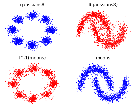
Top left: the data distribution, bottom right: the target distribution. Top right: the data distribution mapped to the target distribution using a learned flow. Bottom left: the target distribution mapped to the data distribution using the inverse of the learned flow.
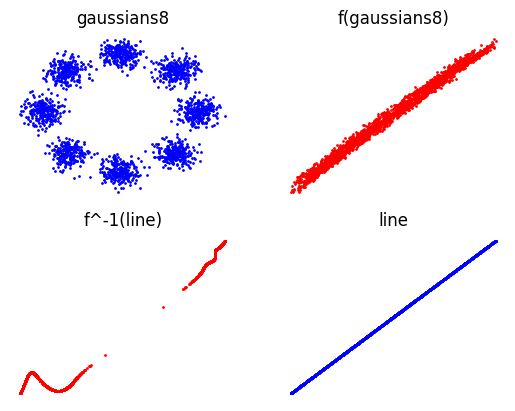
Similar organisation to the previous figure. However we see that the learned flow is not able to map the line to the 8-Gaussian dataset.
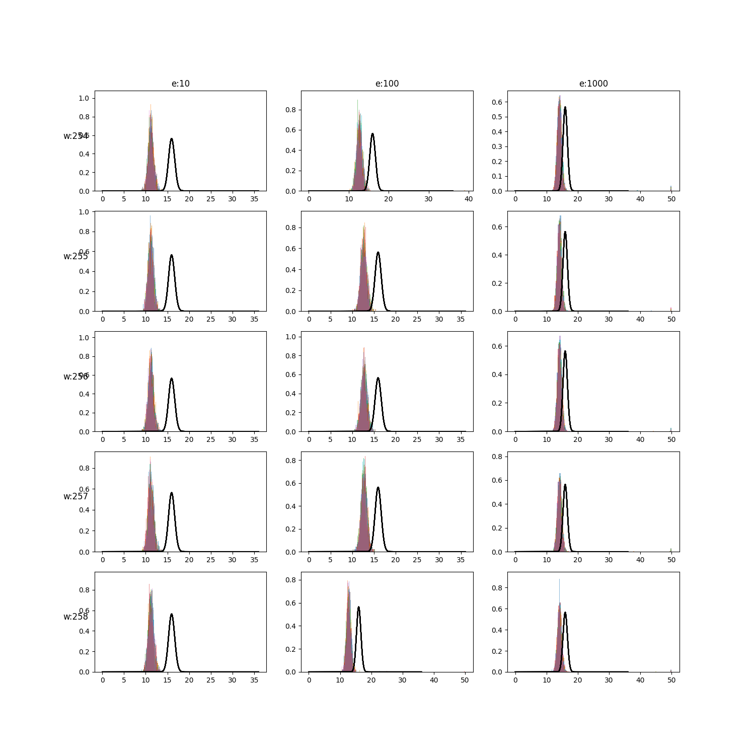
Again, but in higher dimensions we demonstrate this issue. Here we define our data distribution to be a istropoic, zero mean, Gaussian in 64 or 128 dimensions with 0.5 variance. We define our target distribution to be a isotropic, zero mean, Gaussian in 128 dimensions with 1.0 variance.
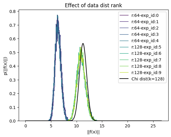
Here we have plotted the histogram of norms of the forward flow, ${\parallel f(x) \parallel: x \in p(x)}$. We have also plotted the Chi distribution, which is the analytical solution to this problem.
In practice this is a problem because many datasets (eg MNIST) do not have 784 dimensions of variation (by computing the rank of the covariance of the MNIST train set we find that it has 228 independent dimensions of variation). Another way of stating this is that the data lie on a low-dimensional manifold.
If we allow ourselves to use randomness, then this problem quickly disappears. Thus why diffusion models do not suffer from this issue.
An alternative solution is to use latent flows. By projecting the data into a lower dimension where all the variation is captured we avoid this issue.
Latent flows appear to be in common use (Dao et al., 2023; Esser et al., 2024), however the reasons for using them is not often understood (other than increases in performance).
Bibliography
- Albergo, M. S., Boffi, N. M., & Vanden-Eijnden, E. (2023). Stochastic Interpolants: A Unifying Framework for Flows and Diffusions. arXiv. http://arxiv.org/abs/2303.08797
- Liu, X., Gong, C., & Liu, Q. (2022). Flow Straight and Fast: Learning to Generate and Transfer Data with Rectified Flow. arXiv. http://arxiv.org/abs/2209.03003
- Lipman, Y., Chen, R. T. Q., Ben-Hamu, H., Nickel, M., & Le, M. (2023). FLOW MATCHING FOR GENERATIVE MODELING.
- Dao, Q., Phung, H., Nguyen, B., & Tran, A. (2023). Flow Matching in Latent Space. https://arxiv.org/abs/2307.08698
- Esser, P., Kulal, S., Blattmann, A., Entezari, R., Müller, J., Saini, H., Levi, Y., Lorenz, D., Sauer, A., Boesel, F., Podell, D., Dockhorn, T., English, Z., Lacey, K., Goodwin, A., Marek, Y., & Rombach, R. (2024). Scaling Rectified Flow Transformers for High-Resolution Image Synthesis. https://arxiv.org/abs/2403.03206