Diffusion is just stacked denoising score matching!
August 10, 2024
Our goal is to approximate a data distribution $p(x)$ with a model $p_{\theta}(x)$ using a set of samples, $D_n = { x_i: x_i\sim p(x), i \in Z_n }$.
With this model of the data distribution we can generate our own samples $x\sim p_{\theta}(x)$, and we can evaluate the likelihood $p_{\theta}(x)$. This ability to sample and evaluate facilitate many tasks in machine learning; generative modelling, density estimation, and anomaly detection.
We start formulating the problem as finding a model distribution that minimises the KL divergence to the data distribution.
\[D_{KL}(p, p_{\theta}) = \mathbb E_{x \sim p(x)} [ \log p(x) - \log p_{\theta}(x) ] \\\]The data distribution term $\log p(x)$ doesnt depend on $\theta$ and can be ignored when optimising $\theta$.
\[\theta^{* } = \text{argmax}_{\theta} \mathbb E_{x \sim p(x)} [ \log p_{\theta}(x) ] \\\]Thus we are maximising the likelihood $p(x \mid \theta)$ of the data under the model. Solving this optimisation problem is hard. There are many different ways we can construct our model, $p_{\theta}(x)$. However, they require that:
\[\int p_{\theta}(x) dx = 1\]This constraint is, in general, intractable. However, if we are clever, we can avoid this constraint. For example;
- normalising flows construct invertible maps (that preserve density) between distributions. Thus, as long as the initial distribution is normalised, the final distribution will also be normalised.
- variational autoencoders attempt to find a latent space where the data distribution is a simple (ie gaussian) distribution.
- energy based models learn an energy function which corresponds to unnormalised probabilities.
In this blog, we consider yet another approach.
Model the score indead of the density
An alternative approach to modelling the density is to approximate the score function, $s(x, \theta) \approx \nabla_x \log p(x)$. This allows us to avoid the normalisation constraint. Note, we can generate samples using a score function by using Langevin dynamics (Welling & Teh, 2011).
Instead of the KL divergence (above) which led us to the maximum likelihood solution, we start with the Fisher divergence (Lyu, 2009).
\[\begin{align*} D_F(p, p_\psi) &= \mathbb E_{x \sim p(x)} \parallel \frac{\nabla_x p(x)}{p(x)} - \frac{\nabla p_{\psi}(x)}{p_{\psi} (x)}\parallel^2 \\ \end{align*}\]This leads to the score matching objective function (Hyvarinen, 2011) by using the log derivative trick.
\[\begin{align*} \mathcal L(\theta) &= \mathop{\mathbb E}_{x\sim p(x)} \parallel s(x, \theta) - \nabla_{x} \log p(x) \parallel^2 \\ \end{align*}\]However, this function contains $\nabla_x \log p(x)$, the true score function, which we do not have access to. Our setting only grants samples from the density.
Fortunately, there are two known solutions to this problem; score matching (Hyvarinen, 2011) and denoising score matching (Vincent, 2011).
Score matching
(Hyvarinen, 2011) show that we can write the gradient of the score matching objective in a way that doesn’t contain the score function. Thus allowing us to estimate the score function without having access to it.
The derivation is as follows;
\[\begin{align*} \nabla_\theta \mathcal L(\theta) &= \nabla_\theta \mathop{\mathbb E}_{x\sim p(x)} \Big[ \parallel s(x, \theta) \parallel^2 - 2 \langle s(x, \theta), \nabla_x \log p(x)\rangle + \parallel \nabla_x \log p(x)\parallel^2\Big]\\ &= \nabla_\theta \mathop{\mathbb E}_{x\sim p(x)} \Big[ \parallel s(x, \theta) \parallel^2 - 2 \langle s(x, \theta), \nabla_x \log p(x)\rangle\Big] \\ \end{align*}\]We epanded the score matching objective (from above). Now, the last term will drop off since it is not a function of $\theta$, thus we ignore it. Now we can use the log derivative trick (1.) and a partial integration trick (2.) to rewrite the second term.
\[\begin{align*} \int p(x)\langle s(x, \theta), \nabla_x \log p(x, \theta)\rangle dx &= \int p(x)\sum_i s(x, \theta)_i \nabla_{x_i} \log p(x) dx\\ &= \int p(x)\sum_i s(x, \theta)_i \frac{\nabla_{x_i} p(x)}{p(x)} dx \tag{1.}\\ &= \int \sum_i s(x, \theta)_i \nabla_{x_i} p(x) dx \\ &= \int \sum_i \nabla_{x_i} s(x, \theta) p(x) dx \tag{2.}\\ &= \int p(x) \nabla_x \cdot s(x, \theta) dx \\ \end{align*}\] \[\begin{align*} \nabla_x \log p(x) &= \frac{\nabla_x p(x)}{p(x)} \tag{1.} \\ \int \nabla_x f(x) \cdot g(x)dx &= \int f(x) \cdot\nabla_x g(x)dx \tag{2.}\\ \end{align*}\]Thus we have:
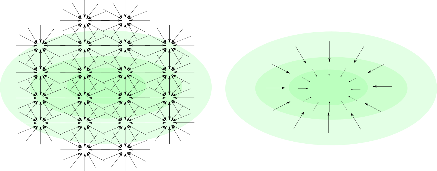
\[\mathcal L_{SM}(\theta) = \mathop{\mathbb E}_{x\sim p(x)} \Big[ \parallel s(x, \theta) \parallel^2 + 2 \nabla_x \cdot s(x, \theta)\Big]\]Let’s try and understand what this objective doing.
The objective is trying to minimise;
- The norm of the score function. This is a regularisation term that prevents the score function from becoming too large.
- The divergence of the score function. This term ensures that the score function is a sink at the data points.
Points with higher density should be larger sinks (to minimise the divergence).
Denoising score matching
Denoising score matching, (Vincent, 2011; Alain & Bengio, 2012) starts by slightly changing the goal. Instead of learning the score function of the data distribution, we learn the score function of a parzen-window density of the empirical data we observe.
\[\begin{align*} q(\hat x) &= \int_x p(\hat x \mid x) p(x) dx \\ &= \int_x \mathcal N(\hat x \mid x, \sigma^2I) p(x) dx \\ &\approx \frac{1}{N}\sum_i^N \mathcal N(x \mid x_i, \sigma^2I) \tag{$x_i\sim p(x)$}\\ \end{align*}\]Our DSM objective function becomes:
\[\begin{align*} \mathcal L(\theta) = \mathop{\mathbb E}_{x\sim p(x)} \mathop{\mathbb E}_{\hat x \sim p(\hat x\mid x)} \parallel s(\hat x, \theta) - \nabla_{\hat x} \log q(\hat x) \parallel^2 \\ \end{align*}\]Since we have chosen our noise distribution to be gaussian, we can calculate the score function of this distribution.
\[\begin{align*} \nabla_{\hat x}\log q(\hat x | x, \sigma) &= -\frac{1}{\sigma^2} (\hat x - x) \\ p(\hat x \mid x, \sigma) &= \mathcal N(\hat x \mid x, \sigma^2I) \\ \nabla_{\hat x}\log \mathcal N(\hat x \mid x, \sigma^2I) &= -\frac{1}{\sigma^2} (\hat x - x) \end{align*}\]Thus our loss becomes:
\[\begin{align*} \mathcal L(\theta) &= \mathop{\mathbb E}_{x\sim p(x)} \mathop{\mathbb E}_{\hat x \sim p(\hat x\mid x)} \parallel s(\hat x, \theta) + \frac{1}{\sigma^2} (\hat x - x) \parallel^2 \\ \end{align*}\]Where the model $s(\hat x, \theta)$ attempts to predict the (normalised) noise added to $\hat x$. Aka, the score function (for additive gaussian noise).
Hopefully the connection to denoisers is clear. Where a denoiser would predict $x$ given $\hat x$, we are predicting the noise added to $\hat x$ given $x$. So it’s possible to extract the score function from a denoiser via
\[s(\hat x, \theta) = \frac{1}{\sigma^2} (\hat x - D(\hat x, \theta))\]Diffusion
What does all this have to do with diffusion?
In diffusion we construct a stochastic differential equation (SDE) that describes the evolution of a distribution over time. (Song et al., 2021)
\[\begin{align*} dx &= f(x, t)dt + g(t)dW_t \tag{forward SDE}\\ dx &= [f(x, t) - g^2(t) \nabla_x \log p(x)_t] dt + g(t)dW_t \tag{reverse SDE}\\ \end{align*}\]The learning objective in to approximate the score, so we can reverse the process.
When discretised, we can view the forward process as
\[p(x_{t+1} \mid x_t) = \mathcal N(x_{t+1} \mid x_t, \sigma(t)^2I) \\ x_{t+1} = x_t + \sigma(t) \epsilon_t \\\]So, to approximate the score function we can use denoising score matching. Undoing the repeated addition of noise.
So we stack many denoising score matching models on top of each other. Each model is trained to denoise the output of the previous model.
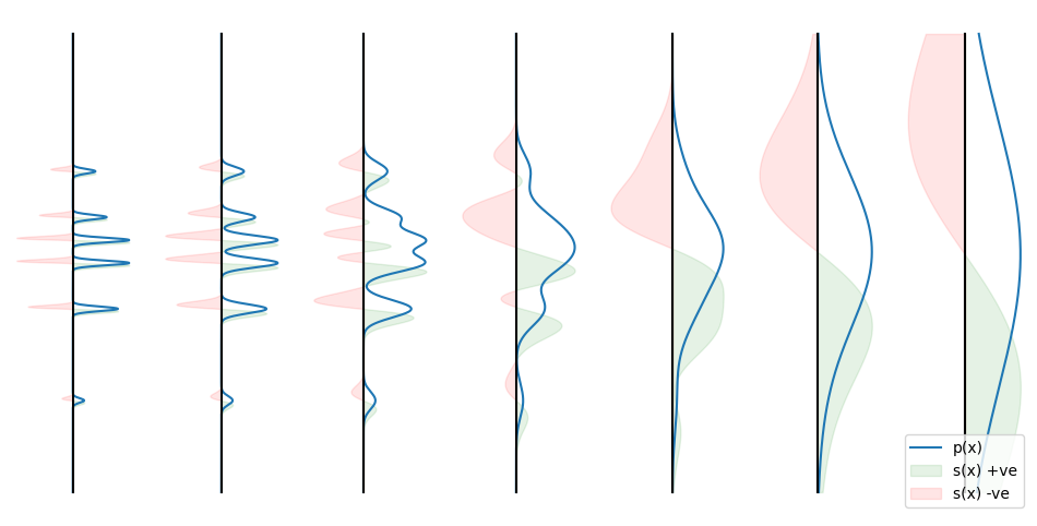
Using this stack of denoisers, we can generate new samples. By taking a sample from a gaussian distribution (right) and passing it through each denoiser. This procedure turns out to be equivalent to doing Langevin dynamics using the score function.
This is cool! Stacked denoisers are much easier to understand than score functions, Langevin dynamics, and SDEs.
Bibliography
- Welling, M., & Teh, Y. W. (2011). Bayesian learning via stochastic gradient langevin dynamics. Proceedings of the 28th International Conference on International Conference on Machine Learning, 681–688.
- Lyu, S. (2009). Interpretation and Generalization of Score Matching.
- Hyvarinen, A. (2011). Estimation of Non-Normalized Statistical Models by Score Matching.
- Vincent, P. (2011). A Connection Between Score Matching and Denoising Autoencoders. Neural Computation, 23(7), 1661–1674. https://doi.org/10.1162/NECO_a_00142
- Alain, G., & Bengio, Y. (2012). What Regularized Auto-Encoders Learn from the Data Generating Distribution (Vol. 15). https://doi.org/abs/1211.4246
- Song, Y., Sohl-Dickstein, J., Kingma, D. P., Kumar, A., Ermon, S., & Poole, B. (2021). Score-Based Generative Modeling through Stochastic Differential Equations. arXiv. http://arxiv.org/abs/2011.13456