In high dimensions, typical is unintuitive
August 10, 2024
What is likely is not (necessarily) typical.
Let’s start with a motivating example: We have a biased coin $p(\text{Heads}) = 0.8$ which we flip $n=100$ times. The most likely outcome is 100 heads, with probability $0.8^{100}=2.037036 \times 10^{-10}$, a small number. So the vast majority of the time, we will observe something else. Most of these other outcomes will be in the range of 70-90 heads. We call these outcomes ‘typical’.
Using the Binomial distribution, we can calculate and plot the probability of getting k heads as;
\[p(k) = \left( 100 \; \text{choose} \; k \right)0.8^k0.2^{100-k}\]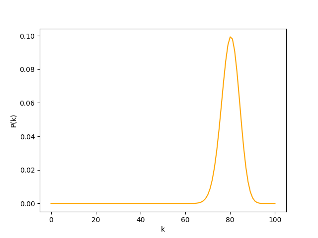
The potentially counter intuitive part being that each individual outcome (with with ~70-90 heads) is less likely than 100 heads, yet, they are the ones we observe.
The explanation is that there is only 1 way to get 100 heads, but MANY ways to get (say) 80 heads ($100 \; \text{choose} \; 80 = 5.3598337 \times 10^{20}$).
Definition (for discrete random variables)
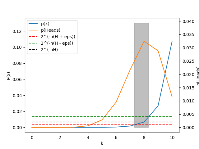
The typical set $\mathcal T (p(x))_{\epsilon}$ is the set of sequences $(x_1,x_2,…,x_n) \in X_n$ with the property
\[2^{−n(H (X)+\epsilon)} \le p(x_1,x_2,...,x_n) \le 2^{−n(H (X)-\epsilon)} \\\]From (Cover & Thomas, 2006) page 59.
So for our coin flipping example, let’s pick $\epsilon = 0.1$ and calculate the typical set.
A more practical example; a survey.
We have a survey with 100 binary questions.
- Do you consider yourself to be a morning or night person?
- Do you prefer cats or dogs?
- Do you prefer tea or coffee?
- Do you prefer to read or watch TV?
- Do you vote left or right?
- … etc
We can collect the data, and we may see that;
- 60% of people consider themselves to be morning people
- 70% of people prefer dogs
- 80% of people prefer coffee
- 60% of people prefer to read
- 30% of people vote left
- etc…
From this data we can construct an archetype of a person who took the survey. This person would be a morning person, prefer dogs, prefer coffee, prefer to read, and vote right. This person is the most likely person to have taken the survey. But they are unlikely to exist! And may not be a good representation of the people who took the survey.
If we rearange the definition of discrete typical sets, we can find a close connection to the definiiton of entropy.
\[\begin{align*} 2^{−n(H (X)+\epsilon)} &\le p(x_1,x_2,...,x_n) \le 2^{−n(H (X)-\epsilon)} \tag{typical set} \\ H (X)-\epsilon &\le -\frac{1}{n} \log p(x_1,x_2,...,x_n) \le H (X)+\epsilon \tag{log both sides} \\ -\frac{1}{n} \log \prod_{i=1}^n p(x_i) &= -\frac{1}{n} \log p(x_1,x_2,...,x_n) \tag{independence} \\ &= -\frac{1}{n} \sum_{i=1}^n \log p(x_i) \\ H(X) &= \lim_{n \to \infty} -\frac{1}{n} \sum_{i=1}^n \log p(x_i) \tag{AEP} \\ &= - \sum_{x \in X} p(x) \log p(x) \tag{entropy} \end{align*}\]Assuming each $x_i$ in the sequence is indpendent and identically distributed (i.i.d) from $p(x)$.
AEP is the asymptotic equipartition property states that for sequences of i.i.d random variables, the mean log probability converges to the entropy of the distribution (Cover & Thomas, 2006) page 58.
Definition (for continuous random variables)
The typical set $\mathcal T (p(x))_{\epsilon}$ is the set of sequences $(x_1,x_2,…,x_n) \in X_n$ with the property
\[\mid - \frac{1}{N} \log p(x) - h(X) \mid \le \epsilon\]Where $h(x)$ is the differential entropy of $p(x)$. (Cover & Thomas, 2006) page 245.
Let’s work through a continuous example. A d-dimensional isotropic Gaussian distribution.
First, we can reframe a d-dimensional Gaussian as sequence of $d$ i.i.d 1D Gaussians. For example, if $d=3$ then we can sample 3 times from a 1D Gaussian to get a sample from a 3D Gaussian.
\[\begin{align*} p(x) &= \prod_{i=1}^d \mathcal N(x_i; 0, \sigma^2) \\ \mathcal N(x; 0, \sigma^2 I) &= \frac{1}{(2\pi \sigma^2)^{1/2}} \exp \left( -\frac{1}{2\sigma^2} x^2 \right) \\ \end{align*}\]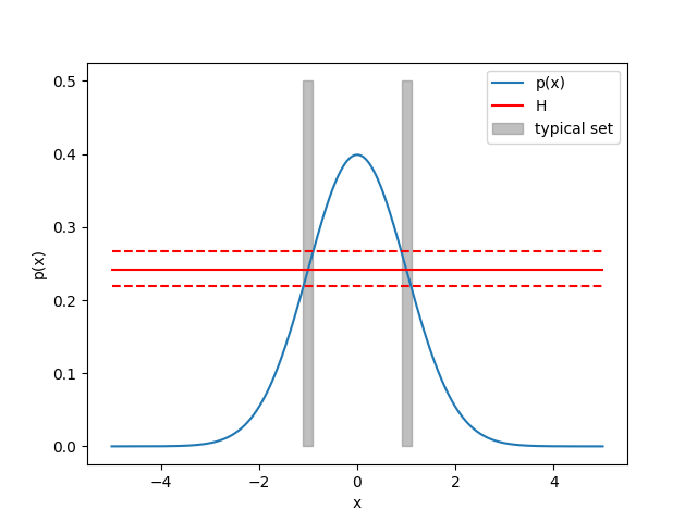
This doesn’t seem to make much sense in 1 dimension. But in higher dimensions, it’s more easy to imagine. If I sample d times from a Gaussian, what’s the chance I get all zeros? Very small. Instead, i’m likely to sample some small numbers, and a few larger numbers. On average, this will yield a sample near the unit sphere. Thus, the typical set is a thin shell around the unit sphere. This is also known as the Gaussian Annulus Theorem.
For a d-dimensional spherical Gaussian with unit variance in each direction, for any $\beta \le \sqrt{d}$, all but at most $3e^{−c\beta^2}$ of the probability mass lies within the annulus $\sqrt{d} - \beta \le |x| \le \sqrt{d} + \beta$, where c is a fixed positive constant.
So high dimensional Gaussian distributions can be imagined as hollow spheres, rather than the bell shaped curves we are used to in 1D.
Much like our discrete example (but replace probability mass with probability density and binomial counts with volume), the most likely outcome has small probability density. And as we move outward, the volume increases exponentially. Thus even though the probability density is small, the volume is large, and we are likely to observe points in this region.
Bibliography
- Cover, T. M., & Thomas, J. A. (2006). Elements of Information Theory (2nd ed.). Wiley-Interscience. https://www.wiley.com/en-us/Elements+of+Information+Theory%2C+2nd+Edition-p-9780471241959