The MAP solution is not the best solution?

MAP produces solutions that are not typical

August 10, 2024

We solve an inverse problem with MAP vs PITS. Here we pick the prior and likelihood to be Gaussian distributions.

\[\begin{align*} p(x) &= \mathcal{N}(0, \sigma_x^2) \\ p(y|x) &= \mathcal{N}(x, \sigma_y^2) \end{align*}\]

Let’s pick the prior to be a Gaussian distribution with mean 0 and standard deviation 1. And the likelihood to be a Gaussian distribution with mean 1 and standard deviation 0.5. We find the MAP solution and the PITS solution.

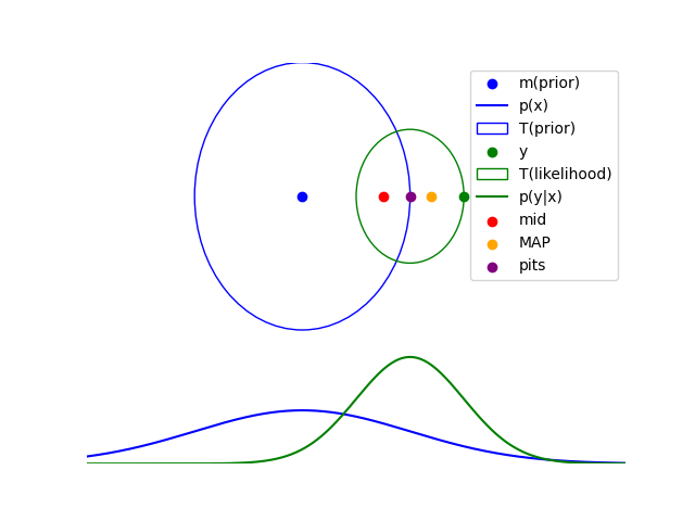
Illustration of the inverse problem for a Gaussian prior and likelihood. Where y is the observation and x is what we want to recover. Top; shows the typical sets of our two distributions and the solutions found by MAP, PITS (where mid is simple the mid point). Bottom; a reminder that we are working with Gaussians.

MAP solution

For Guassian prior and likelihood, can derive the MAP solution in closed form as;

\[\begin{align*} x^*&= \arg \max_x \frac{p(y|x)p(x)}{p(y)} \\ &= \arg \max_x p(y|x)p(x) \\ &= \arg \max_x \log p(y|x) + \log p(x) \\ &= \arg \max_x -\frac{1}{2\sigma_y^2}||y - x||^2 - \frac{1}{2\sigma_x^2}||x||^2 \\ \end{align*}\] \[\begin{align*} \nabla_x \left( -\frac{1}{2\sigma_y^2}||y - x||^2 - \frac{1}{2\sigma_x^2}||x||^2 \right) &= \nabla_x \left( -\frac{1}{2\sigma_y^2}||y - x||^2 \right) + \nabla_x \left( -\frac{1}{2\sigma_x^2}||x||^2 \right) \\ &= \frac{1}{\sigma_y^2}(y - x) - \frac{1}{\sigma_x^2}x \\ &= 0 \\ x^* &= \frac{\sigma_x^2}{\sigma_x^2 + \sigma_y^2}y \\ \end{align*}\]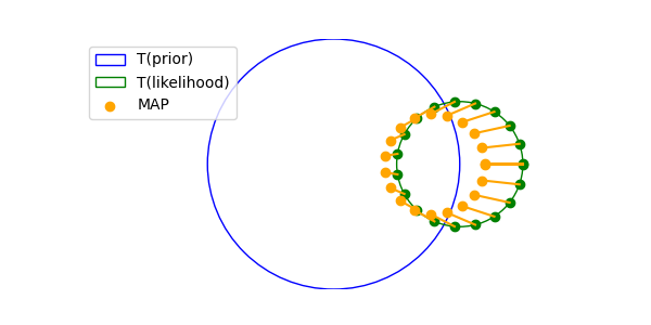

The observed $y$'s are updated to be more likely under the prior.

PITS solution

For Gaussian distributions derived the PITS solution as;

\[\begin{align*} x^* &= \arg \max_{x \in \mathcal T(p(x))_\epsilon} p(y | x) \tag{PITS} \\ &= \arg \max_{x \in \mathcal T(p(x))_\epsilon} \mathcal{N}(x, \sigma_y^2) \\ &= \arg \max_{x \in \mathcal T(p(x))_\epsilon} \exp \left( -\frac{1}{2\sigma_y^2}||y - x||^2 \right) \\ &= \arg \min_{x \in \mathcal T(p(x))_\epsilon} \parallel x - y \parallel^2 \\ \lim_{\epsilon\to 0} \mathcal T(\mathcal N(0, \sigma^2 I))_\epsilon &= \{x ; \parallel x \parallel = \sqrt{d} \sigma \} \\ x^* &= \sqrt{d} \sigma\frac{y}{\parallel y \parallel} \end{align*}\]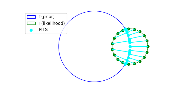

The observed $y$'s are projected into the typical set.

Accuracy

We can compare the accuracy of the MAP and PITS solutions by looking at the mean squared error (MSE) between the true $x$ and the estimated $x$.

\[\text{err} = \frac{1}{N \sqrt{d}} \sum_{i=1}^N ||x_i - x_i^*||^2 \\\]

We find that MAP provides slightly more accurate solutions than PITS. For example, if we pick d=2048, average over 10000 samples. We get an average normalised error of MAP $0.45$ and PITS $0.46$.