Density estimation
Question: Why is density estimation hard? I am not sure. The curse of dimensionality will play a role.
In the previous section we considered VAEs and GANs for density approximation. The deeper problem to the learned prior approach seems to be that we dont have have any methods for efficiently and accurately approximating a density.Maximum likelihood
In an ideal world we would like the ability to approximate arbitrary distributions. To learn $ f: X \to Y $ such that the probability density is preserved. An easy and intuitive way to learn a density model is by maximum likelihood estimation. $$ \begin{align} \hat \theta &= \mathop{\text{argmax}}_{\theta} E_{x\sim D} \left[ p(x, \theta) \right] \\ \end{align} $$Thus, models that allocate higher probability to observed data, the $ x $s, are better. However, the class of functions that $\theta$ can represent is limited. We would like to use an abitrary functon approximator like neural networks, but they fail at maximum likelihood because they can simply predict $nn(x_i) = \infty $ for all inputs. They can do this because they are not normalised.
A simple representation like a tensor that is indexed by possible $x_i$s has a similar normalisation problem (naively optimising it to do ML will give $ \infty $). But, it can be easily constrained/regualised to give normalised results.
$$ \begin{align} p(x) &= T[x] \\ \hat T &= \mathop{\text{argmax}}_{T} \mathbb E_{x\sim D} \left[ p(x)\right] \text{s.t.} \sum_i T_i = 1 \end{align} $$Which might be implemented as simply the decay of each element towards zero probabilty. But, just for mnist $T$ would need have $(28 \times 28)^{256}$ elements for each possible image (which according to Google's calculator is infinity...).
In principle this idea could be applied to neural networks as well. If we increase the probability of a location, it should decrease the probability of other locations. $$ \begin{align} p(x) = \frac{f(x, \theta)}{\int f(x, \theta) dx} \\ \end{align} $$So, how can we efficienty estimate of $\int f(x, \theta) d$ when it is $f$ is a NN. What we want is a parameterised fn that is easily integrated. How about $e^{x}$. Or one that can be decomposed and into simpler parts and integrated analytically.
Alternatively, the point of the normalisation is to ensure large amounts of probability mass are not allocated to unseen data. We could simply take random image samples and train them to have low probability.
Normalising flows
It turns out there is already a vast literature exploring the idea of flexible representations for densities. The main idea can be summarised as: What if instead we could start with a simple distribution and transform it into an arbitrary distribution? $$ p(f(x)) = \frac{1}{det(J(f))}p(x) \\ $$ Using the equation above, we can keep track of how probability density has been stretched or contracted.However, there is a problem. The bijectors (such as $f$ in this case) must be invertible. This means; to generate a (say) 784 dim image, we need to start with a simple distribution also in 784 dims. This doesnt seem ideal, we really want to assume a small number of latent variables generate the high dimensional data.
For some recent work see (Masked autoregressive flows).Heirarchical flows
As hinted at above, the real goal of generative modeling is to learn a hierarchical model. A small set of latent features, in low dimension, generate the high dimensional data we observe. There are two main problem with attempting to construct a hierarchical flow;- transforms that reduce the dimensionality are not invertible.
- the determinant of transforms that reduce (or expand) the demsnsionality is zero (or $\infty$).
(1) Because we assume the data is generated by latent features we are really saying that the data lies on a low dimensional manfold in the higher dimensional space. Thus it possible to have an invertible mapping from said manifold into the latent space. To actually calculate the inverse we can simply use the pseudo inverse.
(2) There is a nice little cheat that allows you to calculate the determinant of a non square transformation. $\det(A) = \sqrt{\det{A\cdot A^T}}$. This calculation matches the usual $\det{A}$ when $A$ is square an is defined when $A$ is not square! Nice.
Effectively both of these come down to calculating the signular value decomposition of our transform and excluding singular values close to zero.
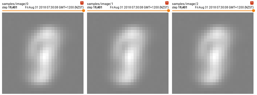
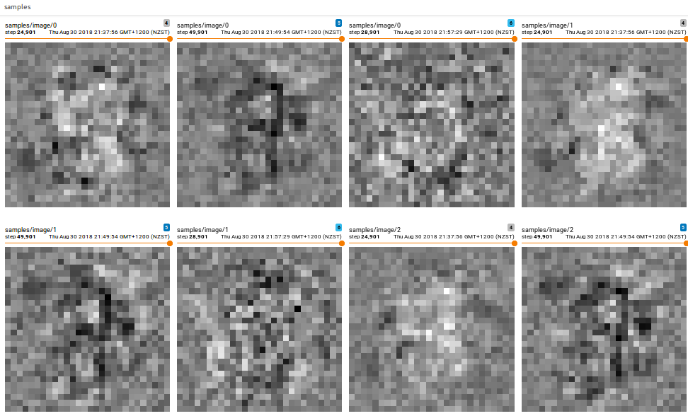
After some initial experiments, it seems like a plasuible idea. The images below show samples taken from a learned density (a simple distribution transformed into a complex one, via a linear transform(s), and learned by maximum likelihood). They definitely seem suggestive.
However, there remain a few important problems (not including the above);
- low probabilty assigned to images at init (how can we init/regularise for uniform dist?)
- non linearities cause p(x) to go to Nan almost instantly
- this algol will not scale to larger images (det and inv will be too slow)