Affirmative Action’s Simplistic Approach

Using a 1-Dimensional Solution for a Multi-Dimensional Problem

The ideal of “equality of opportunity” resonates deeply: the notion that everyone, regardless of their starting point, should have a fair chance to succeed based on their talents and efforts. For decades, affirmative action has been a prominent, often contentious, set of policies and practices aimed at addressing historical and ongoing systemic disadvantages that prevent this ideal from being a reality. Typically, these measures seek to counteract discrimination and promote diversity, particularly in crucial areas like employment and education, by giving consideration to individuals from underrepresented groups.

But our current methods, while well-intentioned, are overly simplistic. In striving for group-level equity, we inadvertently create individual-level inaccuracies and even new forms of discrimination.

What Makes a Rule Discriminatory, Racist, or Sexist?

Before diving into solutions, let’s clarify what we mean. A rule or policy is defined as discriminatory if:

1. It explicitly uses protected characteristics (like race or gender) to treat individuals differently without sufficient justification, leading to disadvantage for some. This is often termed “disparate treatment.”
2. It is facially neutral (doesn’t explicitly mention protected characteristics) but has a disproportionately negative impact on members of a protected group, and this impact cannot be justified by a legitimate, overriding necessity. This is known as “disparate impact.”
3. It relies on overbroad generalizations or stereotypes about groups instead of assessing individual merit, capability, or experienced disadvantage. This is where the “accuracy problem” with some affirmative action proxies comes into play. If a policy assumes all members of Group X are disadvantaged and all members of Group Y are not, it stereotypes and can lead to unfair outcomes for individuals within both groups.

The core of my concern with implementations of affirmative action lies in this third point: the use of broad demographic categories as proxies for individual disadvantage can be inaccurate. And therefore a discriminatory mechanism, even if the overarching goal (rectifying systemic inequality) is laudable.

The Accuracy Problem in Current Affirmative Action

Many affirmative action policies, as they are often implemented and perceived, rely on these broad demographic categories: race, gender, sexuality, or national origin. The underlying logic is that, on average, individuals belonging to certain groups have historically faced and continue to face greater systemic barriers. Therefore, membership in such a group is used as a proxy for having experienced disadvantage.

While it is a true statement on average. To label all individuals within one group as “disadvantaged” and all within another as “advantaged” is a simplification that can feel, and indeed can be, discriminatory. It risks overlooking the struggles of some and unfairly attributing disadvantage (or advantage) to others based solely on a group identity. This isn’t about creating an “oppression Olympics,” but about acknowledging the vast spectrum of individual experiences.

The Single-Variable Predictor: A Technical Analogy of Limited Flexibility

Let’s frame this in more technical, machine learning terms. Imagine we are trying to build a model to predict a latent (unobserved) variable, D_i, representing the “true level of disadvantage” experienced by individual i. Our goal is to use this D_i to inform resource allocation or “plus-factor” considerations.

A common approach in current affirmative action can be likened to a very simple predictive model. Consider trying to predict whether it will rain (Y_rain) using only one variable and two parameters: the percentage of cloud cover (X_clouds).

P(Y_rain = 1 | X_clouds) = σ(β_0 + β_1 * X_clouds)

Where σ is a logistic function (to keep probabilities between 0 and 1). This model has only two parameters (β_0, β_1) to learn. It can only draw a single, simple relationship: more clouds mean a higher chance of rain. It cannot adapt its prediction to other crucial factors. If it’s a cloudy day but the humidity is extremely low and the altitude is very high, this simple model might still predict a high chance of rain, inaccurately. It lacks knowledge (of other variables) and flexibility (more parameters) to adjust its behavior based on a richer set of circumstances.

Similarly, using a single demographic category (X_demographic) to predict “disadvantage” (D_i) is like this simple rain model:

Predicted_D_i = β_0 + β_1 * I(X_demographic = GroupA) + β_2 * I(X_demographic = GroupB) + ...

Where I(...) is an indicator function. This model assigns a fixed level of “average disadvantage” to everyone in GroupA, another to everyone in GroupB, and so on. It has very few parameters (the βs for each group). Its predictions are rigid for individuals within the same group; it cannot tailor its assessment to the unique combination of circumstances that make up an individual’s actual lived experience of opportunity or hardship.

When Do Single-Variable Predictors Work?

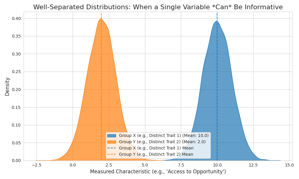
Not all single-variable predictors are inherently flawed for every task. There are situations where relying on a single characteristic can be accurate. This occurs when that single variable is a strong, dominant, and clean signal for the outcome we’re trying to predict.

Consider trying to distinguish between basketballs and golf balls based solely on their diameter.

• Basketballs have a diameter of ~24 cm.
• Golf balls have a diameter ~4.3 cm.

If you were given a diameter, you could predict with extremely high accuracy whether it’s a basketball or a golf ball.

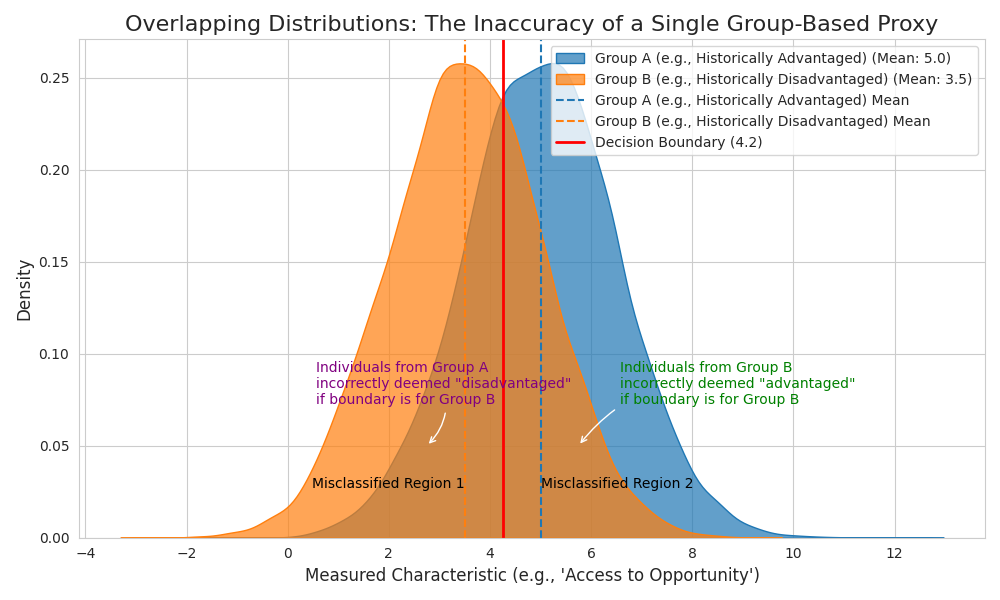
When Don’t Single-Variable Predictors Work?

They don’t work pretty much any time we deal with humans in the real world. We are not as simple as golfballs and basketballs…

How inaccurate are these single-variable predictors in practice? While a universal “inaccuracy percentage” is elusive, studies consistently highlight the limitations:

• Research on “race-neutral” alternatives (which often means substituting race with another single or limited set of proxies like socioeconomic status) indicates they frequently fail to achieve the same levels of racial and ethnic diversity as race-conscious policies. ¹ This suggests these proxies are not adequately capturing the multifaceted nature of disadvantage that race-conscious approaches (however imperfectly) aimed to address.
• In educational data mining, while demographic data is commonly used, its actual value for prediction accuracy is questionable if more direct measures (like student performance or engagement data) are present. ²
• The “proxy problem” is well-documented, where seemingly neutral variables (like zip codes or high school attended) can be so highly correlated with race or socioeconomic status that they effectively replicate the biases of using the protected characteristic directly. ³

The evidence strongly suggests that relying on a single demographic variable as the primary predictor of disadvantage is a statistically weak and ethically problematic approach due to its lack of flexibility and inability to capture individual nuance.

We see this single-variable (or few-parameter) model is inherently limited:

• High Bias: It makes strong assumptions that group membership is the primary driver of disadvantage, ignoring vast within-group variance.
• Low Variance (but misleadingly so): The predictions are stable for members of the same group, but this stability comes at the cost of being consistently wrong for many individuals whose personal experiences deviate from their group’s average.
• Omitted Variable Bias: Crucial factors that determine an individual’s true level of disadvantage are omitted. Research shows that even when demographic variables are excluded, predictive uncertainty can still lead to disparate impacts, with groups having lower average outcomes experiencing higher false negative rates. ⁴

Towards a More Accurate System: The Power of More Parameters and Richer Data

If the single-variable proxy is insufficient, the logical next step is to incorporate more information – to build a richer, more individualized understanding of the opportunities and barriers each person has genuinely faced. In our weather analogy, this means adding more variables like humidity, altitude, wind patterns, temperature, time of year, etc.:

P(Y_rain = 1 | X_clouds, X_humidity, X_altitude, ...) = σ(β_0 + β_1*X_clouds + β_2*X_humidity + β_3*X_altitude + ...)

This model, with more parameters (β_0, β_1, β_2, β_3, ...), has much greater flexibility. It can learn more complex relationships and adjust its prediction based on the specific combination of many factors. It can learn that high cloud cover with low humidity might not mean rain, while moderate cloud cover with high humidity and a certain wind pattern does.

Similarly, for predicting disadvantage, we can move towards a more complex model:

Predicted_D_i = β_0 + β_1*Z_1i + β_2*Z_2i + ... + β_k*Z_ki

Where Z_ji are numerous individual-level factors: socio-economic status of their family and community, quality of schools attended, personal or family health challenges, experiences with discrimination or hardship (e.g., bullying, community violence), access to mentors, networks, and enriching extracurriculars, parental education levels and employment, and so on.

A model with many such parameters gains the flexibility to change its behavior specific to the person, rather than treating them as an interchangeable member of a broad category. Machine learning models, especially complex ones like neural networks or gradient boosted trees, are designed to effectively learn these β weights (or their equivalents) and find intricate patterns in such high-dimensional datasets.

Defining Fairness: A Journey Through Concepts to “Equalizing Mistakes”

Before we unleash ML, we need a clear definition of “fairness.” Let’s walk through some common fairness notions:

1. “Blindness” / “Fairness Through Unawareness”:
   • Idea: Simply don’t use protected attributes (like race or gender) as input features in a decision-making model.
   • Example: A hiring algorithm is designed to predict job success. To be “fair,” it’s not given candidates’ race. However, if the algorithm uses candidates’ zip codes, and zip codes are highly correlated with race due to historical residential segregation, the algorithm might still penalize applicants from certain racial groups without ever “seeing” race directly.
   • Problem: This is often ineffective. Other variables can act as proxies, reintroducing bias. Moreover, ignoring historical context can mean failing to address existing systemic inequalities. It doesn’t guarantee fair outcomes.
2. Demographic Parity (or Statistical Parity / Group Fairness / Same Proportion):
   • Idea: The proportion of individuals selected (e.g., receiving a “plus factor,” loan approval, or job offer) should be the same across different demographic groups. Mathematically: P(Ŷ=1 | A=a) = P(Ŷ=1 | A=a') for all groups a, a'.
   • Example: A university aims for demographic parity in its engineering program admissions. If Group A makes up 50% of the general population, the university decides 50% of admitted engineering students must come from Group A, regardless of the proportion of qualified applicants from Group A for that specific, demanding program.
   • Problem: This can be problematic if the underlying true prevalence of “qualified individuals” (Y=1) actually differs between groups for those specific roles, perhaps due to historical inequities in access to prerequisite education, but there many also be other causes. Forcing equal selection rates could mean selecting less qualified individuals from one group or overlooking more qualified individuals from another, simply to meet a quota. It doesn’t account for whether the selections are correct based on the defined criteria for success in the role/program.
3. Threshold-Based Fairness (e.g., a single threshold for a “risk score”):
   • Idea: Apply the same decision threshold (e.g., a certain “risk score” for recidivism, or a “qualification score” for a loan) to all individuals, regardless of group.
   • Example: If a single risk score threshold (e.g., score > 7 means “high risk,” deny parole) is used for both men and women, it could be unfair to women. If women, on average, have lower actual re-offense rates than men for any given risk score, then applying the same threshold means women might be denied parole at a rate that is disproportionately high relative to their actual risk of reoffending. The score ‘7’ might mean a 60% chance of reoffending for men but only a 30% chance for women. Similarly, if a scoring system for loan applications (where lower scores are worse) on average assigns lower scores to applicants from Group X than Group Y for reasons unrelated to their actual likelihood of repayment (e.g., due to biased data), applying the same approval score threshold to both groups would unfairly disadvantage applicants from Group X. ⁵
   • Problem: If the score itself is biased or if the meaning of the score (i.e., the probability of the actual outcome given the score) differs systematically across groups, then applying a single threshold will still lead to unfair outcomes.

This brings us to a more robust set of definitions, focusing on equalizing error rates, as discussed by Kearns and Roth and central to algorithmic fairness research:⁵

1. Equal Opportunity:
   • Idea: Among all individuals who genuinely should be identified (e.g., Y=1, truly experienced significant disadvantage, or are truly qualified for a loan/job), the probability of being correctly identified (Ŷ=1) should be the same across all groups g \in G.
   • Mathematical Definition: P(Ŷ=1 | Y=1, G=a) = P(Ŷ=1 | Y=1, G=a') for all groups a, b \in G'.
   • Example: In a hiring context, let Y=1 represent candidates who would be successful if hired. Equal opportunity would mean that if 80% of truly capable candidates from Group A are correctly identified and offered a job by the algorithm, then 80% of truly capable candidates from Group B should also be correctly identified and offered a job. It ensures the system doesn’t have a higher false negative rate (missing qualified people) for one group compared to another.
   • This focuses on ensuring the True Positive Rate (TPR) is equal. It means the system doesn’t disproportionately make false negative errors (failing to identify someone who should be identified) for one group over another. This is crucial for ensuring that those who genuinely merit consideration are not overlooked due to their group affiliation.
2. Equalized Odds:
   • Idea: This is stricter. It requires both the True Positive Rate (TPR) AND the False Positive Rate (FPR) to be equal across groups. The FPR is the probability of incorrectly identifying someone as Y=1 when they are truly Y=0.
   • Mathematical Definition:
     • P(Ŷ=1 | Y=1, G=a) = P(Ŷ=1 | Y=1, G=a') (Equal TPR)
     • AND P(Ŷ=1 | Y=0, G=a) = P(Ŷ=1 | Y=0, G=a') (Equal FPR)
   • Example: Continuing the hiring example: Equalized Odds requires that the algorithm not only correctly identifies successful candidates at the same rate across groups (equal TPR) but also incorrectly identifies unsuccessful candidates (i.e., makes bad hires) at the same rate across groups (equal FPR). So, if 5% of candidates from Group A who would not be successful are mistakenly offered a job (a false positive), then 5% of candidates from Group B who would not be successful should also be mistakenly offered a job.
   • This means the system is equally likely to make both types of mistakes (false positives and false negatives) for all groups. It aims for a balance where no group is unduly burdened by either type of error. Research indicates that without careful intervention, predictive models often assign higher false negative rates to lower-average groups and higher false positive rates to higher-average groups. ⁴

If our current, proxy-based affirmative action systems were audited against Equalized Odds, it’s highly plausible they would fail, making different types of mistakes at different rates for different groups due to the crudeness of the proxies. The goal of a more sophisticated, ML-driven approach would be to strive for something like Equalized Odds, using a rich set of individual features rather than broad demographic categories as the basis for affirmative action.

Can Machine Learning Build Fairer Systems? The Promise and The Perils

The allure of machine learning is its potential to analyze vast, complex datasets and identify subtle patterns that humans might miss or be unable to process. A model fed with rich, individualized data points (socio-economic background, educational history, health indicators, community factors, etc.) could, in theory:

• Develop a more accurate, individualized “disadvantage score” or likelihood of benefiting from an intervention, thanks to its flexibility in handling many parameters.
• Be explicitly optimized to satisfy fairness criteria like Equalized Odds or Equal Opportunity across carefully defined groups.

However, the path is fraught with significant challenges:

1. Biased Data, Biased Models: This is a critical issue. ML models learn from the data they are given. If historical data reflects existing societal biases (e.g., if certain groups were systematically under-supported or discriminated against, leading to poorer outcomes that are then recorded as “less potential”), the model will likely learn and perpetuate these biases, even if the explicit protected attributes like race or gender are removed. ⁶
2. Defining and Quantifying “Disadvantage”: This is perhaps the most profound challenge. What factors constitute “disadvantage”? How should they be weighted? Who decides? These are deeply ethical and societal questions that data science alone cannot answer. The very act of choosing what data to collect and how to label it embeds values and potential biases.
3. The Proxy Problem Revisited: Even if we exclude explicit demographic data, other variables can act as proxies for them. For instance, zip code can correlate strongly with race and socio-economic status. ³ An ML model might inadvertently use these proxies to replicate old biases.
4. Privacy Concerns: Collecting and using the kind of detailed personal data needed for such a system raises immense privacy issues. Secure storage, ethical usage, and individual consent are paramount and incredibly complex to manage.
5. Transparency and Explainability (XAI): Many advanced ML models are “black boxes.” If a model denies someone an opportunity or doesn’t flag them for a “plus factor,” understanding why is crucial for accountability and trust. Fields like Explainable AI are working on this, but it’s an ongoing challenge. ⁷
6. The “Last Mile” Implementation: Even if a “perfectly fair” algorithm could be designed, how its outputs are used in real-world decision-making processes (e.g., college admissions, hiring) is a complex policy and logistical hurdle. Who oversees these systems? How are errors appealed?

Conclusion

The core argument is this: affirmative action policies that rely predominantly on single, broad demographic categories are, in essence, the most rudimentary form of attempting to level an uneven playing field. While the intention to assist those who have faced systemic disadvantages is commendable, this one-dimensional approach is inherently limited in its accuracy and fairness at the individual level. We are using the simplest possible tool for an incredibly complex task.

We can, and should, do much better. The pursuit of true equality of opportunity demands a more sophisticated, nuanced, and individualized understanding of the barriers people face. Leveraging richer data and the analytical power of modern tools like machine learning offers a pathway toward systems that are more accurate in identifying need and more equitable in their outcomes.

References